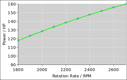
Figure 1: MAP and Power
Copyright © 2008 jsd
Let’s start with the basic equation (as given in reference 1) for flow through an orifice plate, as a function of pressure:
| (1) |
were
We can invert equation 1 to obtain:
| (2) |
where the pressure drop ΔP is given by
| (3) |
where T is the absolute temperature. The second line was obtained using the ideal gas law.
From here on, we measure things in units such that A=1, ρ=1, and T=1 at sea level in the standard atmosphere.
We now make the approximation that flow through the system is isothermal. There won’t be any Joule-Thompson cooling because the air is very nearly ideal. There could be some slight adiabatic cooling, because the air is moving faster on the downstream side. But there could also be some heating, because of the proximity of the hot engine. All in all, at this level of detail, we’re not going to worry about it. Our temperature T will fall off with altitude in accordance with the standard atmosphere model.
Plugging into equation 2 with m• = ρ2 U• and ρ2 = MAP/T we obtain:
| (4) |
which is all very nice except that it has MAP on both sides of the equation. Writing it as a quadratic in standard form we have:
| (5) |
where
| (6) |
Roughly speaking J scales directly like flow squared, and inversely like throttle area squared.
Solving for MAP/A we find
| (7) |
and we drop the ± sign because only the positive root makes sense. The expression O(⋯) is “Big O” notation as described in reference 2. For example, √(1+x) = 1 + x/2 − x2/8 + O(x3).
The first line of equation 7 tells us that when J is large, MAP/A goes to zero, and asymptotically it scales like J−0.5, or equivalently like a/U•.
The second line was obtained by expanding the square root to second order. It tells us that when J is small, i.e. when the flow is small and the throttle is wide open, MAP starts out equal to A and then drops off linearly as a function of J, i.e. quadratically as a function of U• and/or inverse quadratically as a function of a.
Equivalently we can write
| (8) |
The indicated power Ei• will scale like U• times the density ρ2, and we approximate ρ2 as MAP/T, which gives us
| (9) |
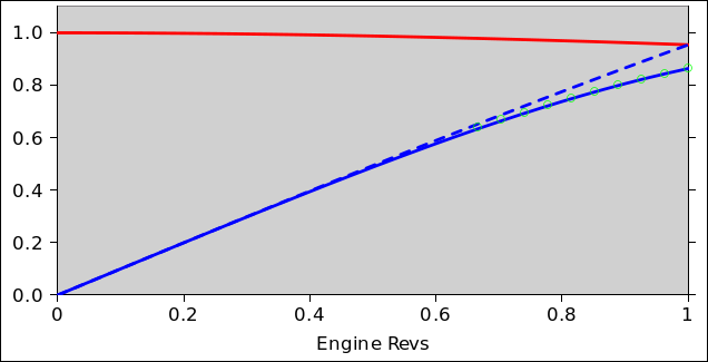
In figure 1, the red curve represents the MAP in accordance with equation 7. The dotted blue curve represents the indicated power in accordance with equation 9.
We can compare this against data from a real engine, via the Lycoming O-320 Operator’s Manual, as shown in figure 2.
Referring back to figure 1, the real-engine data is shown by the green circles. The data has been scaled horizontally so that redline revs (2700 RPM) maps to 1 in the local units. Similarly the data has been scaled in the vertical direction to match the local units. That is necessary because 1.0 local units of power corresponds to a purely hypothetical situation, as if the MAP were boosted all the way up to ambient.
There is a pretty good fit between our model and the Real World data. This shouldn’t be taken as proof that the model is correct in all respects; the RW data is almost linear and there must be a huge class of models that can be tweaked to match the data. On the other hand, it is clear that the RW data cannot be used as evidence against our model.
Now let’s consider an example situation that can easily arise in an aircraft with a fixed-pitch prop. At the beginning of the takeoff roll, the engine rotation rate is relatively low. Then, as the aircraft rolls down the runway, picking up speed, the revs increase. Our equations tell us that under “normal” full-throttle conditions, this increase in revs means the engine increases its power output. The increase is less than proportional, but under any conditions where the MAP remains reasonably high (as shown by the red curve) it is almost proportional.
The indicated power curve in figure 1 is monotonic, as it should be in this high-MAP situation ... although as we shall see in section 1.6, at low power and high rotation rate it can become non-monotonic.
You can compare and contrast these curves with the data presented in reference 3, reference 4, and reference 5. Note that reference 5 contains a copy, probably the ancestral copy, of the nomogram for “Sea Level and Altitude Performance”.
In equation 1 and equation 6, the factor K represents everything that is not changing, i.e. everything that does not depend on revs, temperature, or throttle setting. This includes things like the volumetric displacement of the engine, the overall size of the throttle valve, various constants of nature, and various conversion factors for the units involved.
To say the same thing in more mathematical terms, in equation 6, we see that J depends on several factors, all of which get multiplied together. Therefore we can trade off one factor against the other. In particular, if we change the units of measurement for the area a, the flow rate U•, and/or the temperature T, we can make up for it by changing the factor K appropriately.
In typical modeling situations, we don’t know the area of the full-open throttle. This means we can’t do any ab initio calculations, and makes it convenient to simply normalize a so that a=0 represents “throttle closed” and a=1 represents “throttle full open”.
While we are at it, we might as well normalize U• so that U•=1 represents max rated revs (multiplied by the displacement of the engine), and normalize T so that T=1 is the absolute temperature at sea level (under standard day conditions).
Using normalized values for a, T, and U• is harmless if we are willing to adjust K. In practice, we adjust K to get a plausible MAP under known conditions.
As a way of estimating K, we bring in some Real World data from e.g. a PA-28-180 that indicates that a MAP of 28.5 inHg is reasonable, at full throttle and max rated revs. This corresponds to ΔP/A = 0.05 and hence J = 0.1
| (10) |
which would imply, for this engine,
| (11) |
This is the value of K2 used to construct the curves in figure 1 and figure 4.
Here “lossess” refers to friction and other processes that remove energy from the system, reducing the available power and reducing the thermodynamic efficiency. In contrast, “deductions” cause the available power to be less than it might have been without reducing the thermodynamic efficiency, as discussed in section 1.6.
Here are some of the possible contributions to internal losses that should be considered:
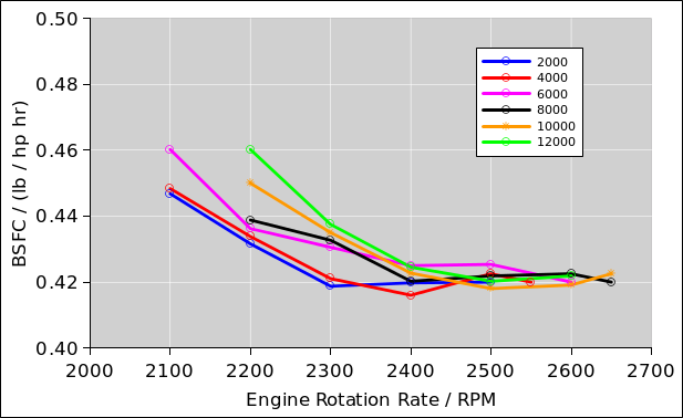
We will soon discuss each of these contributions in more detail. However, you may wish to skip the details, because it turns out that none of this matters. Our discussion of these losses must remain, at least for now, theoretical and hypothetical, because there is no evidence that they significant in any particular engine. They are all phenomena that should be more pronounounced at high revs, but when we look at data for a Real World Lycoming O-320 engine, the inefficiency (as measured by BSFC, brake-specific fuel consumption) gets worse at low revs, as shown in figure 3.
By the way, the Lycoming BSFC data is not as bad as it looks in figure 3. Part of the ugliness in the figure is due to roundoff errors. The data came to me (via Cessna) suffering from overly aggressive roundoff.
You can probably skip this section.
We now consider the following:
Any leftover combustion products in the cylinder will interfere with the introduction of new fuel/air mixture. Leftovers will be more prominent at high revs, because there is simply less time available to complete the scavenging process.
Similarly, the charging of the new fuel/air mixture may be less than 100% complete at high revs, again because there is less time.
These processes do not contribute much to thermodynamic inefficiency, because whatever fuel/air mixture does enter the cylinder can still be used efficiently.
We will not attempt to construct a first-principles physics model for these phenomena, but we can cook up a phenomenological model. The data tells us that the shaft power scales like revs times MAP except for a slight downturn at high revs. We model this by throwing a factor of (1−αU•3) into the power equation, where α is some small constant, adjusted to make the model match the performance of real engines.
An example of all how this plays out can be seen in the solid blue curve back in figure 1. The deduction stands out as the difference between the dotted blue curve and the solid blue curve.
In figure 1, the deduction seems only moderately large. However, if we take the same engine to a higher altitude (lower ambient pressure), or close the throttle most of the way, then the indicated power is much less, and the deduction at any given rotation rate is just as large, so the effect is a larger portion of the total. This can be seen in the lowest blue curve in figure 4, which is non-monotonic: it peaks when the abscissa (engine revs) is 0.73 in the local units.
We now consider the effect of using the throttle.
We assume the throttle-knob θk somehow controls the area a of the orifice.
We know that the throttle valve never completely closes, even when the throttle knob is pulled “all the way” out. So we can write
| (12) |
where we assume that θk is normalized to lie in the range [0,1] and therefore θv lies in the range [i,1], where i is some sort of “idle” setting. We further assume that the geometry of the throttle has been engineered so that a ∝ θv2.
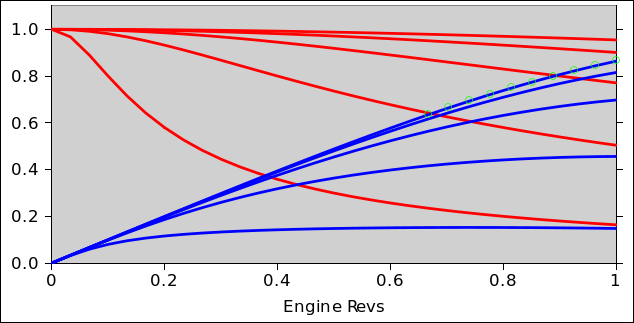
The effect of the throttle is summarized in figure 4. There are five different blue curves, one for each throttle knob setting in the set {0, .25, .5, .75, 1.0}, showing the power. The red curves show the corresponding MAP. For these curves, the idle is set at i=0.2.
The power curves in figure 4 include some deductions as discussed in section 1.6. In fact, the top red curve and top blue curve in figure 4 are identical to the solid curves in figure 1.
Consider the following scenario: The SW (Sim World) c182rg is sitting on the runway at KSFO. The propeller control is pulled back, so that the engine is operating at relatively low revs, about 1750 RPM in contrast to redline which is 2400 RPM. The pilot can observe that if the throttle is open anywhere between 52% and 100% open, moving the throttle has no effect on the MAP. Similarly, it has no effect on the shaft power of the engine, as you can confirm by looking at the property tree. This insensitivity to throttle setting is dramatically unlike what is seen in a RW (Real World) Cessna 182RG.
This unrealistic behavior can be taken as a purely phenomenological observation. Unadorned observation is sufficient to demonstrate that the behavior of the SW aircraft is unrealistic.
Alternatively, or additionally, we can try to understand the misbehavior as a consequence of the model used by FlightGear version 1.99.5-rc2, as implemented in FGPiston.cpp. The code for MAP is
    suction_loss = RPM > 0.0 ? ThrottlePos * MaxRPM / RPM : 1.0;
    if (suction_loss > 1.0) suction_loss = 1.0;
    MAP = p_amb * suction_loss;
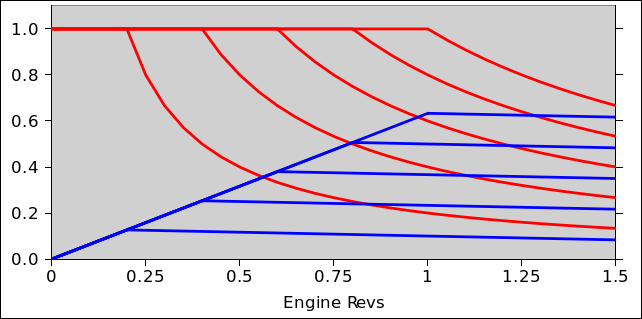
The results created by this code are shown in figure 5. Once again the red curves represent MAP. From that I have derived the power (blue curves) by multiplying by rotation rate, and then subtracting off a friction term.
In the figure, observe that when the revs are 0.5 in the local units, three of the five throttle settings have the same MAP and the same power. That is to say, moving the throttle will move you from one blue curve to another, but since three of the five blue curves lie one atop the other, this has no effect. Ditto for the red curves. This agrees with the in-the-cockpit observations of the unrealistic SW behavior.
We can compare and contrast figure 5 with figure 4. In particular, in figure 4 we see the following fundamental trends:
You can see that figure 5 mimics these trends to a degree, but only crudely and qualitatively.
One could start by redoing our analysis, replacing A (the ambient static pressure) by the compressor’s upper-deck pressure. That’s super-easy. The tricky part is to account for the energy spent driving the turbine. I don’t have any numbers on that. That number is not normally displayed on the instrument panel, neither in cars nor in airplanes.
The model is more general, in that it deals with arbitrary throttle settings and arbitrary engine rotation rates. It contains the Gagg-Farrar result as an approximate corollary in the special case where the rotation rate U• is held constant and of course the throttle setting remains constant.
We can see how this comes about via equation 9. The dominant contribution to the fall-off, at constant revs, is the ambient density term A/T. There is an additional dependence on altitude via the factor of T in the definition of J, which enters equation 9 as a smallish correction term, which is not captured by the Gagg-Farrar formula.
Copyright © 2008 jsd