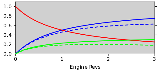
Figure 1: Plot of 1/(1+x) and x/(1+x)
Copyright © 2008 jsd
Let’s start with the basic equation for fluid flow versus pressure drop in a pipe:
| (1) |
were V• is the volumetric flow rate at the inlet, Z is the flow impedance, µ is the dynamic viscosity, and ΔP is the pressure drop.
This equation properly applies when the pressure drop is not very large, but we are going to abuse it by applying it even when the pressure drop approaches 100% of the inlet pressure. As a consequence, the results will be only approximate, but that’s better than nothing, and better than unguided guessing.
The SI unit for dynamic viscosity µ is the pascal·second (Pa·s). The dynamic viscosity of air is mildly sensitive to temperature but insensitive to pressure and density at constant temperature. At 15∘C it is µ=1.8 Pa·s and at 0∘C it is µ=1.7 Pa·s.
We are interested in the case where ΔP represents the drop across the induction system, including the air cleaner, the throttle, the carburetor, and the induction manifold. In this case we can write
| MAP = A − µ Z V• (2) |
where MAP is the manifold absolute pressure, and A is the ambient static pressure.
We now make the approximation that flow through the system is isothermal. I suspect it is closer to adiabatic (isentropic), but for first-draft purposes let’s stick with isothermal. Then by conservation of mass we can write
| (3) |
where U• is the volumetric flow within the manifold, i.e. on the downstream side of the impedance. Recall that V• is the volumetric flow on the upstream side of the impedance. We assume that to a fair approxmation U• is the rate at which volume is pumped through the engine, so it scales like the displacement times the rotation rate.
Plugging in this expression for V• into equation 2, we get
| MAP = A − µ Z U• MAP / A (4) |
and solving for MAP we find
| MAP = |
| (5) |
The indicated power Ei• will scale like U• times density, which we approximate by U• times MAP, which gives us
| (6) |
It is worth taking a moment to explore the implications of this expression. For starters, we observe that if the ambient pressure remains constant and the throttle impedance remains constant, this is a simple function of U•. In fact it is is a nondecreasing function, as you can see from the blue curve in figure 1.
Here is a situation that can easily arise in an aircraft with a fixed-pitch prop. At the beginning of the takeoff roll, the engine rotation rate is relatively low. Then, as the aircraft rolls down the runway, picking up speed, the revs increase. Our equations tell us that the power increases. The increase is less than proportional, but under any conditions where the MAP remains reasonably high (as shown by the red curve) it is almost proportional.
The indicated power curve in figure 1 is monotonic, but we shall see in section 1.3 that at low power and high rotation rate it can become non-monotonic.
The next step is to account for internal losses in the engine. This means that the shaft power of the engine will be less than the indicated power calculated above.
The main contributions to internal losses are
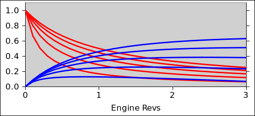
We model the losses as proportional to RPM. An example of how this plays out can be seen in the dotted blue curve in figure 2.
In this example, the effect of friction is not terribly large. However, if we take the same engine to a higher altitude (lower ambient pressure), then the indicated power is much less (as shown by the solid green curve in figure 2) and the friction at any given rotation rate is just as large, so the effect of friction is a larger portion of the total. Indeed, in this regime, the shaft power is no longer a monotonic function of rotation rate, as shown by the dotted green curve, which peaks when the rotation rate is about 1.7 in the local units.
We now consider the effect of using the throttle.
To a first approximation, the impedance will depend inversely on the openness of the throttle valve, θv, that is:
| Z ∝ 1 / θv (7) |
But we know that the throttle valve never completely closes, even when the throttle knob is pulled “all the way” out. So we can write
| (8) |
where we assume that θk is normalized to lie in the range [0,1] and therefore θv lies in the range [i,1], where i is some sort of “idle” setting.
| MAP = |
| (9) |
where β is just the viscosity combined with some proportionality factors.
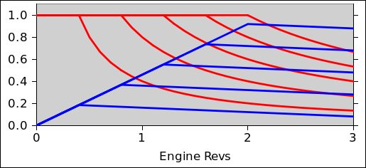
The effect of the throttle is summarized in figure 3. There are five different blue curves, one for each throttle knob setting in {0, .25, .5, .75, 1.0}, showing the power. Similar the red curves show the MAP. For these curves, the idle is set at i=0.2.
The curves in figure 3 include some internal losses as discussed in section 1.3.
As a sanity check, we consider the edge case where the throttle is closed θk=0 and assuming i is small. This gives us:
| (10) |
So we see that the idle-power is rather sensitive to ambient pressure. It’s quadratic. This is not surprising, but does make an interesting contrast with the full-throttle power, which is closer to being a linear function of ambient pressure. You can see this by taking the low-Z limit of equation 6. A linear fall-off in Ei• is basically the Gagg-Farrar result.
You can see in more detail how this comes about by writing A = 1 + є where є is small. In practice є will be negative but that does not affect the calculation we are about to do. Plugging this into equation 6 we get:
| (11) |
The point of all that is as follows: When Z is small (wide open throttle), the coefficient in front of є is close to 1, which means indicated power falls off linearly as a function of ambient pressure ... while when Z is large (throttle nearly closed), the coefficient in front of є is close to 2, which means the fall-off is quadratic.
The physics here can be understood as follows: When Z is large, we need two factors: one factor of pressure to push a volume of air through the impedance, and then the aforementioned factor of density, to tell us how much mass was in that volume. When Z is small, the only thing that matters is the density, and the volume is determined by the displacement of the engine.
Consider the following scenario: The Sim World c182rg is sitting on the runway at KSFO. The propeller control is pulled back, so that the engine is operating at relatively low revs, about 1750 RPM in contrast to redline which is 2400 RPM. The pilot can observe that if the throttle is open anywhere between 52% and 100% open, moving the throttle has no effect on the MAP. Similarly, it has no effect on the shaft power of the engine, as you can confirm by looking at the property tree. This insensitivity to throttle setting is dramatically unlike what is seen in a Real World Cessna 182RG.
This unrealistic behavior can be taken as a purely phenomenological observation ... or we can try to understand it as a consequence of the model used by FlightGear version 1.99.5-rc2, as implemented in FGPiston.cpp. The code for MAP is
    suction_loss = RPM > 0.0 ? ThrottlePos * MaxRPM / RPM : 1.0;
    if (suction_loss > 1.0) suction_loss = 1.0;
    MAP = p_amb * suction_loss;
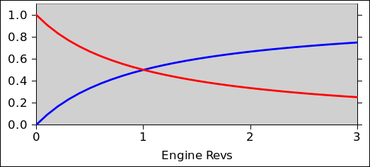
The results created by this code are shown in figure 4. Once again the red curves represent MAP. From that I have derived the power (blue curves) by multiplying by rotation rate, and then subtracting off a friction term.
In the figure, observe that when the revs are 1 in the local units, three of the five throttle settings have the same MAP and the same power. That is to say, moving the throttle will move you from one blue curve to another, but since three of the five blue curves lie one atop the other, this has no effect. Ditto for the red curves.
We can compare and contrast figure 4 with figure 3. In particular, in figure 3 we see the following fundamental trends:
You can see that figure 4 mimics these trends to a degree, but only crudely and qualitatively.
The model is more general, in that it deals with arbitrary throttle settings and arbitrary engine rotation rates. It contains the Gagg-Farrar result as a corollary in the special case where the impedance Z is negligible and the rotation rate is constant.
Copyright © 2008 jsd