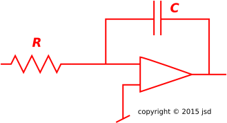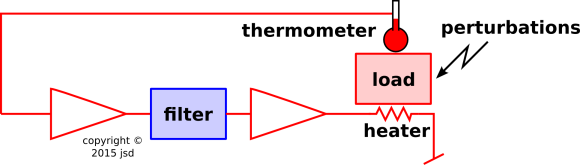
Figure 1: Temperature Controller System
Here’s the basic outline. We start with two simple but important ideas:
|
The classic example of negative feedback is a thermostat. If things get too cold, the thermostat turns on the heater.
Designing a Linear Control System requires understanding the physics of the heater, load, and thermometer, in order to figure out what sort of filter we need to achieve optimal control.
Let’s consider the idea of feedback as a function of frequency. Assume the system is reasonably linear, so we can analyze it component by component. Here’s another key idea, not entirely obvious, but super important:
Now consider the amplitude. Inject a small perturbation into the system somewhere – anywhere – and chase it around the loop back to where you started. That is the operational definition of loop gain. A positive loop gain of less than one means that the perturbation dies out eventually. If it’s close to one it might make several trips around the loop before dying out, but that’s more-or-less tolerable. It means that the perturbation gets magnified by a finite amount, like leverage. On the other hand, if the loop gain is positive and bigger than one, the control system fails completely. The perturbation grows without bound. If this is a DC perturbation, the system locks up. If it is AC, it oscillates like crazy. The oscillations grow exponentially until the system goes nonlinear and/or catches fire.
You can see where this is going: We want a lot of loop gain at DC (to minimize the long-term error) but if there is any kind of delay in the system we need to roll off the gain in such a way that it satisfies the Nyquist criterion:
As a corollary, it is provably impossible to build a perfect feedback loop. If things are changing slowly, the feedback loop can do an excellent job of detecting and nullifying the changes. However, if there is a sudden shock to the system, the feedback loop will need some time to figure it out.
The Nyquist criterion is sufficient to guarantee stability. It is not quite necessary-and-sufficient, but you would be well advised to uphold this condition, unless you are an expert doing something super-unusual.
So, for present purposes, that’s the whole story. Everything else is just a bag of tricks for keeping track of what the phase and amplitude are doing.
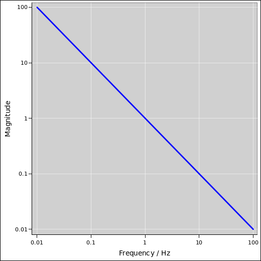
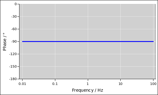
Consider the analog integrator circuit shown in figure 2.
The integral of sine is minus cosine, i.e. 90 degrees delayed. Also the magnitude of the integral is inversely proportional to frequency. The magnitude and phase for an ideal integrator are plotted in the following graphs.
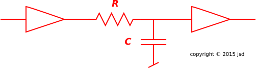
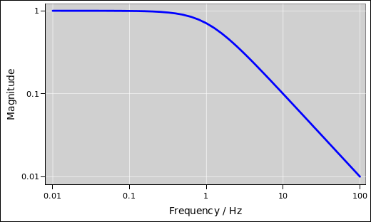
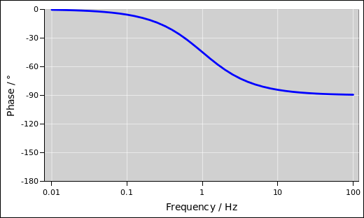
Consider the simple RC low-pass filter shown in figure 5.
This filter has a gain that decreases as a function of frequency. It also has a phase that depends on frequency. At low frequencies the output is in phase with the input, but at high frequencies the thing looks like an integrator, and the output lags the input by 90 degrees. This is shown in the following figures.
That’s what we call a one-pole filter. If you don’t know what a pole is don’t worry about it.
Note that a so-called RC filter does not have to be made of electronics. It could involve a thermal conductivity together with a heat capacity.
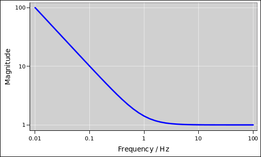
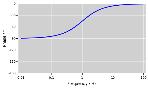
The same goes for integrators. If you have something with a big heat capacity and excellent thermal insulation, it tends to act like another low-pass filter. The temperature goes like the integral of the heat input.
At low frequencies, it looks like an ideal integrator. At high frequencies, it looks like a simple direct proportionality. In the regime where it acts like an integrator, there is a 90∘ phase lag, just like we saw in section 2.1. In the proportional regime, the phase lag goes away.
You can also have a circuit that functions as a differentiator, especially at low frequencies.
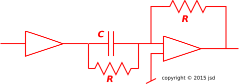
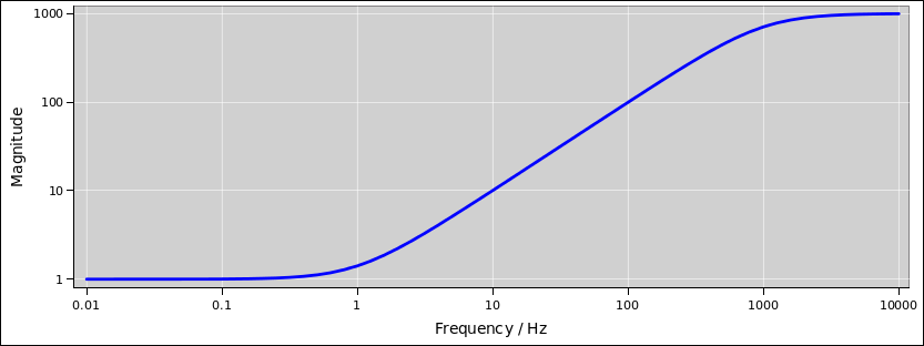
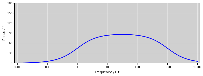
Rather than show that, let’s skip directly to a circuit that contains a differential term plus a proportional term, as shown in figure 10.
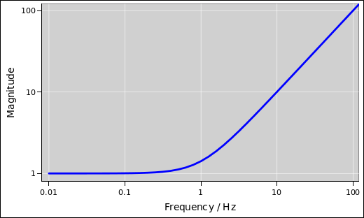
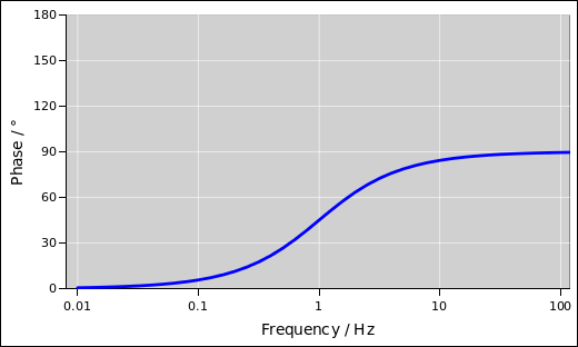
It will act like a simple proportionality at low frequencies, but act like a differentiator at higher frequencies. Note that in the regime where it acts like a differentiator, you get a phase lead, not a phase lag.
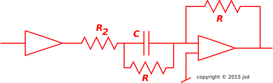
Such a thing is too good to be true. If it kept going like that, it would put out infinite power at infinite frequency. In real life, you have to put an upper bound to the frequencies that can be differentiated. The result looks like the following:
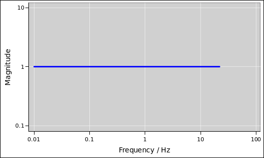
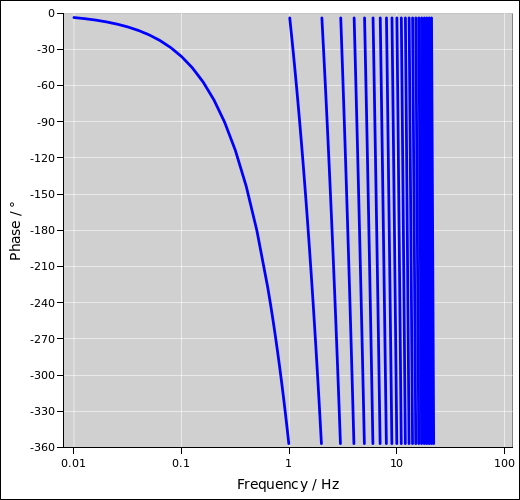
Simply delaying a signal introduces a phase lag proportional to frequency. It reaches 90∘ of phase lag at a frequency of 0.25/t, where t is the amount of delay. When plotted on log/log axes, it’s a spectacular mess:
Let’s see if we can understand the principles behind a P-I-D temperature controller. That stands for proportional-integral-differential.
Before we get started, note that not every controller is of this type. The thermostat in your house is not P-I-D. It’s barely even P. It doesn’t control the temperature very closely, but people don’t seem to mind. In contrast, there are other situations, especially in the science lab, where you want to control something very closely.
Conversely, it should also be noted that not all P-I-D controllers are temperature controllers; see section 4.3.
Be that as it may, let’s start by considering a generic temperature controller. If it exerts only proportional control, i.e. heat proportional to the temperature error, then there will always be some error, in proportion to the amount of heat needed. You can get rid of that by integrating the error, and applying heat according to the integral of the error, but that introduces 90 degrees of phase shift. The integral of sine is minus cosine, i.e. 90 degrees delayed.
Now we have a problem, because there is 90 degrees from the integrator plus 90 degrees from the thermal RC, which is enough to take it right to the edge of oscillating, and if there is the slightest additional delay anywhere the system will really and truly oscillate.
So, we want a component that acts like an integrator below the RC corner frequency, but proportional above – something like we saw in section 2.4. This can be formalized in terms of a pole at zero hertz plus a zero at the 1/2πRC frequency. The zero in the controller cancels the pole in the thermal RC filter. This is a P-I controller. At this point you have a loop gain with effectively one pole at zero Hz and nothing else. That’s good. That’s 90 degrees of phase shift at all relevant frequencies. If that’s all there is, you can turn up the loop gain as high as you want and everybody is happy as clams.
To say the same thing another way, figure 8 multiplied by figure 6 makes figure 3. That means we don’t have 90 degrees from the integrator plus 90 degrees from the thermal RC; instead we have one or the other, for a total of 90 degrees everywhere.
This explains the “P-I” in a P-I-D controller. The pure integrator curve as shown in section 2.1 is about the best you can hope for with analog electronics, without getting ridiculously complicated. One pole gives you 90 degrees of phase shift and enough roll-off that you can have arbitrarily large gain at low frequencies, and still get below unity gain at higher frequencies. With no poles, you would have high gain at all frequencies, and have no chance of satisfying the Nyquist criterion. With two poles, you would have 180∘ of phase shift, which is already too much. So one pole is baby-bear just right.
This leaves us with two unanswered questions, which turn out to be related: How high can we turn up the loop gain? And what about the “D” in the P-I-D controller?
The final key idea is that there is always “something else” to worry about ... some other sources of phase shift ... not just the thermal RC time constant. There will always be lots of other time constants in the system. For starters, I guarantee you that each op-amp has a finite gain-bandwidth product. A circuit such as figure 10 can oscillate all by itself, without even being connected to the thermal system we are trying to control. Similarly, any digital filter introduces some delay, and delay creates phase lag.
As an extreme example, illustrating how thermal controllers can get into trouble: Suppose you are trying to control the temperature of a robot on Mars. If you send a command to the heater, you won’t observe any effect for a number of minutes, for reasons having nothing to do with the thermal conductivity 1/R and the heat capacity C.
We can figure out the optimal strategy as follows: On a minute-to-minute bases, we can operate open-loop, that is, with no feedback at all, using only feed-forward tactics. The information we already have is the only information we are going to get for a long time. However, we are not helpless. We know the observed temperature and we know the desired temperature. We also know the heat capacity. So we send the heater the command to turn on for a certain amount of time and then turn off again, so as to deliver the appropriate amount of energy. That is a perfectly reasonable open-loop feed-forward strategy.
This looks somewhat like a derivative, in the following sense: We saw a step-function error in the temperature, and to a first approximation we commanded a delta-function power output from the heater. It’s not really a derivative, because the heater can’t put out a delta function. It can, however, put out a blip of power, an approximate delta function, with the correct area under the curve.
We can combine that with feedback, by redefining what we consider the error signal to be. We are not particularly concerned by the discrepancy between what the robot is doing right now and the commands we are sending right now; we are much more concerned by the discrepancy between what the robot is doing right now and the commands we sent several minutes ago. Again this looks like a derivative, because we are subtracting the expected result from the observed result, with a time delay. It’s not exactly a derivative, but it’s qualitatively similar.
So we see that the “D” in the P-I-D temperature controller is a bit of a misnomer, but it’s in the ballpark. In any case, it has got precious little to do with the thermal properties of the system. If the thermal RC were the only consideration, a P-I controller would work just fine. However, there is always something else. Sometimes you don’t need super-optimal performance, but if/when you do, you will be tempted to turn up the loop gain to get quicker response and more precise control ... and the only thing that limits the gain is some junk effect, e.g. some delay, some bandwidth limit, some slew-rate limit, or whatever. If you are lucky, one of these effects will dominate the others. It will contribute only one more pole. You can nullify that pole by dropping a zero on it, and that’s what the “D” term in the P-I-D controller does. The pseudo-differentiator in figure 14 has a zero at 1Hz and a pole at 100 Hz, so it doesn’t really reduce the number of poles. It does however buy you an additional two orders of magnitude. Remember, you are busy rolling off the gain at -6 dB per octave (by means of a pole zero hertz), so pushing the crucial second pole out by a factor of 100 in frequency means you can increase the loop gain by a factor of 100. This is not infinite, but it’s a worthwhile improvement.
Beware that there are less-favorable situations where something that looks like a simple differentiator is not good enough. For example, rather than having one dominant junk effect, there could be a whole zerg of them. Ten things contributing 10∘ of phase apiece is 100∘. The properly operating loop has 90∘ of phase shift, so adding another 100∘ is a disaster. What’s worse the rate-of-change of phase with respect to frequency is ten times worse than what you’d get from a single pole, so even if you could fix the phase with a differentiator, it wouldn’t stay fixed. Similarly a plain old differentiator is nowhere near sufficient to deal with round-trip delay to Mars. There are things you can do, but they require something much more sophisticated than a differentiator. They require a detailed model of what the problem is ... which is sometimes available and sometimes not.
In case it wasn’t obvious from the previous discussion:
There exist systematic methods for measuring the loop gain in a feedback system while it is running. This allows you to see whether or not the loop is properly tuned up. Among other things, it allows you to see how close you are to violating the Nyquist criterion, before you actually violate it. The techniques are elegant and clever, but not widely known. For analog circuits, this requires you to have some instrumentation that isn’t too widely available ... phase sensitive wave analyzers and such. For digital filters, it is possible to build “virtual instrumentation” into the software, but sometimes people aren’t clever enough to do this, so you are left even more in the dark than you would be with an analog filter.
Explaining how this works is waaay beyond the scope of this document. It is the sort of thing that gets covered in a semester-long upper-division engineering course.
Beware that not everything in this world is linear. Suppose you have a nice linear thermometer, and a nice linear control system that puts out a voltage related to the temperature error in the usual P-I-D way. If you run that voltage into a heater, you’ve got big problems, because the heater power goes like the square of the voltage. This can easily lead to situations where the system is stable when the errors are small, but unstable when they are large. Just when you think it is working, it fails catastrophically.
In such a situation you would be well advised to take the square root of the voltage before applying it to the heater. This is easy to do in software. It’s tricky but doable in analog circuitry.
Not all P-I-D controllers are temperature controllers. Forsooth, the first automatic P-I-D controllers were developed to help with the steering of ships.
You can of course steer a ship without fancy circuitry, but still there is a feedback loop. The helmsman is part of the feedback loop. Even a not-very-large vessel has enough yaw-axis inertia to make life miserable for the helmsman ... and with an unskillful helmsman you can get quite spectacular oscillations.
A similar situation arises in airplanes. A student pilot can easily cause wild oscillations around the pitch axis. This is so common that there’s a conventional name for it: PIO (pilot induced oscillation). The pitch axis has some natural aerodynamic feedback of its own, and the response time is comparable to human reaction time, so if you combine the two you get more than enough phase shift to violate the Nyquist criterion.
Similar things happen when flying in cloud, flying by reference to instruments. a name for that too: Chasing the needle. This is particularly miserable with the “classic” instruments, because the sensitivity of the needle varies over a tremendous range, so the loop gain is changing. You need quite a sophisticated mental model to deal with this.
Newton’s second law says that the position is the second integral of the force, so if you are observing the position and controlling the force, you’ve got two poles at zero frequency. You’ve got 180∘ of phase shift before you even get started, and it just gets worse from there. This is much nastier than a thermal RC, which is only one pole.
There are two obvious ways of combatting oscillation in such systems. The first is to turn down the gain. That is, figure out how much you want to move the control, and then move it half that much. Wait to see what happens. If it’s not enough, you can add more later.
The more sophisticated way is to apply feedback to the velocity, not just the position. For example, on a ship, if the desired heading is to the right of the present heading but there is a big rate of yaw toward the right, your first priority is to stop the rate. This may require left rudder, even though the desired heading is still well to the right of the current heading.
The same logic applies in airplanes: Stop the needle. That is, look at the velocity of the needle, and make that one of the main inputs to your mental feedback loop.
We can understand the importance of velocity feedback using the same principles. In accordance with Newton’s laws, the position is two integrals removed from the force. That’s two poles at zero hertz. That’s a horror show, if you’re trying to build a simple feedback loop, applying a force in proportion to the position error. In contrast, the velocity is only one integral removed from the force. So you can apply a force in proportion to the velocity, and use that to make a nice stable feedback loop.