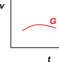
Figure 1: Velocity versus Time
There are many variations in the terminology used to describe velocity and acceleration. In order from good to bad, we have:
Here is my attempt to present the basic equations in a way that is self-consistent, reasonably standard, and reasonably tasteful.
We start by defining acceleration in terms of the rate-of-change of velocity:
| a := |
| (1) |
That can be rearranged to give:
| dv = a dt (2) |
We can approximate differentials by finite differences, which gives:
| Δv = a Δt (3) |
where by definition
| (4) |
where t1 is some “reference time” and v1 is the velocity at that time.
Equation 3 is exactly equivalent to equation 2 if the acceleration is uniform, and is a good approximation if the interval [t1,t] is small enough that the acceleration doesn’t change too much during the interval.
Plugging the definition of Δv into equation 3, we obtain
| v = v1 + a Δt (5) |
and then plugging in the definition of Δt we obtain
| v = v0 + a t (6) |
where we have introduced
| v0 := v1 − a t1 (7) |
which is the velocity at time t=0 (not to be confused with the velocity at time t=t1, except in the special case where t1=0).
We could have made equation 4 look prettier and more symmetric by putting subscripts on v and t, perhaps like this:
| (8) |
However, that would saddle us with unwanted subscripts in later equations. So there are three options:
Option (c) is my least-favorite; I disfavor using two names for the same thing, especially when there is no good reason for it. (However, that is nowhere nearly as bad as using the same name for two different things!) Option (a) is slightly inferior to option (b), on the grounds that an artist should make the final result look good, even if the intermediate stages don’t look very good.
(On the other hand, one could imagine that in slightly different circumstances, it would have been worthwhile to have subscripts on everything.)
For several reasons, we do not write:
| ☠ v = v(t) ☠ (9) |
For starters, the v on the LHS of equation 9 would have a different meaning from the v on the RHS. One of them is a variable, while the other is a function. There’s no way v could be both a variable and a function, as suggested by equation 9. It would be better to write:
| v = G(t) (10) |
where v (as always) is a variable, t is a variable, and G is a function, i.e. a set of ordered pairs.
Let’s be clear: We are using v as a variable and t as another variable. Together they span the (t,v) plane. The expression (t,v) is an ordered pair. The term abscissa by definition refers the first member of such a pair, while ordinate refers to the second member.
A function is, by definition, a set of ordered pairs such that for each abscissa there is a unique ordinate. The red curve in figure 1 is an example of a function, i.e. a set of (t,v) pairs.
Another problem with writing v = v(t) is that it is ambiguous. We don’t know how to evaluate v = v(13). Does the RHS refer to Δt=13 in accordance with equation 5, or does it refer to t=13 in accordance with equation 6? We can solve this problem by defining
| (11) |
where the v is the same v on both lines of equation 11, but G has a different functional form than H.
Properly speaking, there is a function that gives us v in terms of t. We call this function G in accordance with equation 11. The function is not properly called v. We use v to denote a typical point in the range of G, and use t to denote a typical point in the domain of G.
When people speak less precisely, they oftentimes say v is a function of t when they mean v is known in terms of a function of t. That is, they use the name of the ordinate as a shorthand for the name of the function. This is very common, but it is sloppy shorthand. It can get you into trouble in cases where there are multiple ways of computing v.
On the other side of the same coin, people commonly say v is not a function of t when they mean there does not exist any function that gives v in terms of t. Again, they are using the name of the ordinate as a shorthand for the name of the function. This is sloppy shorthand, and it can get you into trouble.
It is a deep principle of physics that the fundamental laws of physics remain the same over time. Therefore if we define
| τ = t + 100 (12) |
then any fundamental law written in terms of t should be equally valid – and have exactly the same form – when written in terms of τ. This can be considered a form of gauge invariance, namely time-shift invariance. Using t corresponds to one choice of gauge, while using τ corresponds to a different choice of gauge. You can choose any gauge you like, so long as you use your chosen gauge consistently. Also keep in mind that others folks may choose differently.
It is worth noting that equation 1, equation 2, and equation 3 are all manifestly invariant with respect to time-shifts. That’s because the differential operators and the delta operators annihilate any shifts or offsets.
In contrast, other equations (notably equation 6) do not exhibit time-shift invariance. That’s OK because they are non-fundamental; they are corollaries of the more-fundamental equations. In writing equation 6, we have already exercised our freedom to choose what we mean by t=0. Having done so, we cannot freely change our mind. If we wanted to apply an offset to t, i.e. to shift what we mean by t=0, we would need to recalculate the value of v0.
According to Galileo’s principle of relativity, the fundamental laws of physics are invariant with respect to an offset in the velocities, such as occurs if one observer is moving relative to another observer. That is, if we define
| u = v + 100 (13) |
then any fundamental law written in terms of v should be equally valid – and have exactly the same form – when written in terms of u.
It turns out that equation 1, equation 2, and equation 3 manifestly exhibit Galilean invariance.
In contrast, the other equations (notably equation 6) do not exhibit Galilean invariance. That’s OK because they are non-fundamental. In writing equation 6, we have already exercised our freedom to choose the state of motion of our reference frame. Having done so, we cannot freely change our mind. If we wanted to switch to a different reference frame that is moving relative to the first, we would need to recalculate the value of v0.