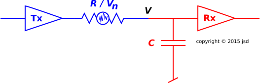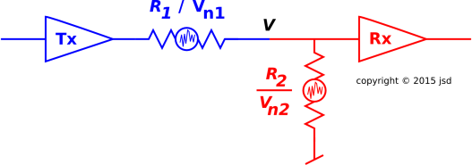
Figure 1: Resistor/Resistor Noise Divider
In electrical circuits, the noise due thermal fluctuations in a resistor is called Johnson noise. Some important applications are discussed in section 4.
The question arises, what happens if there are two resistors in parallel? How much noise does the combination produce? That question is particularly interesting because there are two different ways of answering it. It is amusing to do it both ways and think about why two calculations that look so different produce the same result.
The Johnson noise is well described by the famous Nyquist formula:
| (1) |
where V is the voltage, kT is the temperature (in energy units), B is the frequency (in circular measure, not radians), and R is the resistance. The brackets ⟨⋯⟩ denote an ensemble average.
Algebraically, equation 1 could hardly be simpler, although conceptually you have to think about it for a while before you really understand it. It is a direct consequence of the laws of motion and basic thermodynamics, i.e. the idea that there is ½kT of thermal energy per quadratic degree of freedom, combined with a clever way of enumerating the degrees of freedom in the resistor.
Johnson and Nyquist were colleagues; they published back-to-back papers in The Physical Review in 1928 (reference 1 and reference 2).
We will not rederive the Nyquist formula here. Instead, we take it as a starting point and investigate some of the consequences. In section 2 we explore what happens when there are two resistors are in parallel. Then in section 3, we explore what happens if there is a capacitor in the circuit, resulting in a frequency-dependent noise voltage.
Consider the circuit shown in figure 1. Circuits like this show up all the time. We can consider R1 to be the output impedance of the line driver (Tx), while R2 is the input impedance of the receiver (Rx). The Tx triangle itself is an ideal zero-impedance voltage source; whatever impedance is associated with the driver is included in R1. Similarly, the Rx triangle itself is an ideal infinite-impedance voltage measuring device; whatever input impedance is associated with the receiver is included in R2.
Suppose that Tx is putting out zero volts, so that the only voltages in the system are the noise voltages. We are particularly interested in the voltage V at the point where the two subsystems meet. Note that this voltage appears directly at the input to the Rx triangle.
The Johnson noise in R1 is a distribution over voltages. In accordance with equation 1, the distribution is characterized by the mean square voltage, namely:
| (2) |
A similar formula applies to R2.
We start by considering the limit where R1 is very large compared to R2. That means the noise voltage associated with R1 is very large. However, that voltage gets reduced by a factor of g, where g is less than 1 and represents the “gain” of the voltage divider formed by R1 and R2, namely:
| (3) |
Reducing the voltage by a factor of g reduces the mean square voltage by a factor of g squared. So all in all, the contribution to V from R1 is:
| (4) |
In the limit where R1 becomes large, its contribution becomes negligible. The only noise we see comes from R2. Qualitatively this makes sense; an infinite resistor is equivalent to an open circuit. It might as well not be there.
The two resistors play completely symmetrical roles. The corresponding formula for the contribution from R2 is:
| (5) |
Now we need to add these two contributions. If we knew the voltages, we would just add them, but we don’t. All we have is a statistical distribution over voltages. Taking the square root of equation 4 or equation 5 will not tell you “the” voltage; instead it tells you the width of the distribution over voltages.
Adding uncorrelated random voltages means the widths will add in quadrature. So, the distribution on V is characterized by a mean square voltage:
| (6) |
There is another way of figuring out the noise voltage. We could just recognize that the effective resistance is the parallel combination of R1 and R2:
| (7) |
We use the Nyquist formula directly to calculate the noise in this resistor:
| (8) |
Using a little algebra, you can confirm that equation 6 and equation 8 are equivalent.
Discussion: The most important part of the calculation is realizing that it can be done in more than one way!
It is amusing that two wildly different methods of calculation arrive at the same answer, namely equation 6 which agrees with equation 8. This didn’t happen by accident. It is connected to some fundamental principles of thermodynamics.
For one thing, it is important to look closely at the starting point. In figure 1, we assumed that the two resistors were in thermal equilibrium with each other. Thermodynamics tells us that subject to mild provisos, equilibrium is isothermal. That is to say, two objects in thermal equilibrium are at the same temperature. Even though the resistance-values are different, the temperatures are the same (at equilibrium). The main proviso is that each object must be big enough and complicated enough to serve as a “heat bath” for the other. For reasons explained in reference 2, if you include the resistor and the heat sink to which it is bolted, it makes an extraordinarily good heat bath.
Furthermore, we have the idea of equivalent circuit. If R1 in parallel with R2 is equivalent to Reff – equivalent for the purposes of Ohm’s law – the theoretical model in reference 2 says it should be equivalent for the purposes of thermodynamics also. It should have the same density of states, and therefore the same fluctuations. If equation 6 did not match equation 8, it would tell us that the model was wrong.
This is how a good bit of theoretical physics gets done: You find something that can be calculated two different ways, and compare the results. Most of the time the results agree, but if they disagree you’ll learn something by figuring out why.
Another example of calculating something two different ways leads to equation 12 in section 3. Among other things, that tells us that the factor of 4 in equation 1 is not a mistake; it is the only possible value that is consistent with fundamental notions of thermodynamics.
We now turn to the resistor/capacitor voltage divider in figure 2. This is different from the situation we considered in section 2, because the capacitor divides the noise voltage coming from R but does not add any noise of its own.
As always, the noise in R is a distribution over voltages, as given by equation 2. This is a linear circuit, so we can analyze it frequency by frequency. At any given frequency f, the voltage that appears at node V will be less Vn by a factor of
| (9) |
Putting the ingredients together, we find that the noise at node V in any band B is:
| (10) |
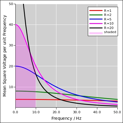
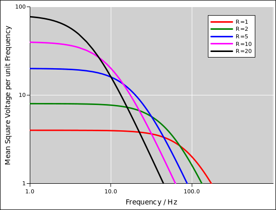
The noise density (i.e. the integrand in equation 10) is shown in figure 3 for a fixed capacitor and various different resistor values. Figure 4 shows the same data on log/log axes.
The integral in equation 10 can be expressed in terms of the arctangent. Integrating it from zero to the corner frequency f0 gives f0 π/4. Integrating it from zero to infinity gives f0 π/2, which is exactly twice as much. The shaded region in figure 3 is half of the total area under the magenta curve.
| (11) |
where the last line is, remarkably enough, independent of the resistance. We have an RC circuit, and the physical origin of the noise is in the resistor, but the magnitude of the noise is independent of the resistance, for any circuit of this kind.
In other words, the area under the curve is the same for all curves in figure 3. For our example circuit, the area is 200π in the appropriate units. That’s because we have chosen kT=1 and chosen the capacitor value to be .01/2/π. Those values were chosen so as to make the corner frequencies come out to be round numbers when expressed in hertz.
In particular, since the resistance does not appear in the last line of equation 11, we are free to consider the case where R → ∞, which is a capacitor all by itself. In this case the noise density curve (as in figure 3) becomes a delta function; there is a distribution of voltages at zero frequency and nowhere else. That is to say, the voltage on the capacitor is not fluctuating, but if we take an ensemble of capacitors, there will be a spread in voltage. The average energy on the capacitor is
| (12) |
which agrees with basic notions of thermodynamics.
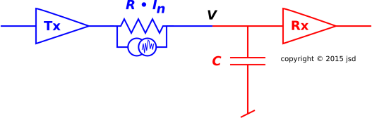
Note that it is always possible to replace a noise voltage in series with a noise current in parallel. Compare figure 5 with figure 2.
The mean square noise current is inversely proportional to resistance. Compare equation 13 with equation 2.
| (13) |
This is consistent with Ohm’s law: A current proportional to 1/√R, multiplied by R, gives a voltage proportional to √R.
This gives us another way to understand the large-R behavior of the circuit in figure 2. The capacitor is fed by a very small noise current. The capacitor integrates this current over a very long time. If you wait long enough, the charge on the capacitor will random-walk a very long way ... but you do have to wait.
Johnson noise is relevant in a tremendous variety of circuits. This is an example of how thermodynamics applies in real-world situations.