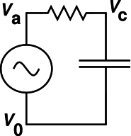
Figure 1: RC Circuit
Let’s start by saying a few words about why it’s worth paying attention to linear circuits, and paying attention to how the circuit responds to sine-wave inputs.
Certain circuit elements including resistors, capacitors, inductors, transformers, batteries, delay lines, antennas, and wires are called linear. That means the voltage drop across the device is a linear function of the current through the device, and vice versa. Of course nothing is exactly linear, but ordinary devices are often nearly so, near enough for a wide range of practical purposes. That means that any signal-processing circuit you build out of such devices will have an output signal that is a linear function of the input signal. This should be obvious from the fact that a linear function of a linear function is itself a linear function.
Linearity implies superposition. That is, if the input is a sum of two functions, the output will be a sum of two functions:
| (1) |
The famous Fourier theorem says that any reasonably well-behaved periodic function can be approximated as a sum of sine waves.
Combining this with the superposition principle (equation 1), we see that if we understand how the circuit responds to sine waves, we know essentially everything there is to know about the circuit. We can analyze it one frequency at a time, and then add up the results.
Just to keep things in perspective, we should mention that some elements are highly nonlinear. This includes diodes, light bulbs, and logic gates.
It should also be emphasize that even when the voltage and current are linear functions of the input, the power will be a nonlinear function. Typically the power depends in nontrivial ways on the voltages and currents at all frequencies, not on each frequency separately. This is usually not much of a problem. Then first step is to calculate all the voltages and currents. Do this for each frequency separately, then combine all the contributions in accordance with equation 1. Then, after all the dust has settled, calculate the power directly from the definition.
In the context of a periodic signal, especially a sinusoidal signal, is conventional to define the phase ϕ(t) as:
| (2) |
We see at once that ϕ(0) ≡ ϕ0 is the phase at time t=0.
Beware that it is moderately common to see ϕ0 referred to as «the» phase. This is not the definition. It is a dirty trick. You can get away with it in certain special cases, such as:
Furthermore usually the reference is obvious or well-standardized, in which case we can drop the Δ and drop the word relative, and just call it “the” phase.
Examples include the the phase and amplitude of the gain function. This includes the overall gain (final output versus original input) as well as various other gains (including loop gain, open-loop gain, and closed-loop gain in a feedback system).
Bottom line: In general, there is a distinction between the total phase ϕ(t) and the initial phase ϕ0. You can gloss over the distinction in special cases, if-and-when you are sure it doesn’t matter.
As we shall see, it is often very convenient to express the real voltage V as the real part of a complex number V̂. Specifically:
| (3) |
where ℜ indicates the real part (of everything to its right). This V̂ is called a phasor, as described more fully below. Now ℜ is a linear operator, and multiplication by a scalar such as exp(iωt) is linear. That means they commute with any other linear operator. If you have a linear circuit and you want to calculate some function F (such as the input/output relation), then
| (4) |
which means that you can do the entire calculation in terms of the phasor V̂ and then find the actual voltage at the very last step, by multiplying by exp(iωt) and taking the real part.
It turns out to be very much simpler to keep track of a single complex number V̂ than to keep track of the amplitude and phase of the real voltage V, since amplitude and phase are nonlinearly related to the actual signal.
Be sure to heed the limitations and caveats in section 4.5 and section 4.6.
If the real voltage V has a sinusoidal waveform, it can always be written in the form:
| (5) |
for some real amplitude A, angular frequency ω, and phase φ0.
Equivalently we can write
| (6) |
where ℜ indicates the real part (of everything to the right), and CC stands for complex conjugate (of everything to the left). The sign convention is such that positive ω is what we call positive frequency. This sign convention is consistent with the more-or-less universal practice of writing the impedance of a capacitor as Z= 1/iωC, as discussed in connection with equation 13.
We can expand the exponential, so as to separate out the dependence on φ0:
| (7) |
So we have rederived the trigonmetric identity for the cosine of a sum. Note the minus sign on the last line. The fact is, if you choose zero phase to correspond to a cosine (not a sine) as in equation 5, and then you increase the phase by 90 degrees, you get a negative sine wave. This is an inescapable trigonometric fact.
This allows us to introduce the real-vector phasor representation:
| (8) |
where V1 and V2 can be considered the components of a two-dimensional vector. We call this vector the phasor representation of V. By comparison to equation 7, we can express the phasor components in terms of the amplitude and phase:
| (9) |
which can be inverted as:
| (10) |
The sign convention is such that when V1 and V2 are both positive, it corresponds to a positive frequency. The phasor (V1, V2) = (0, 1) is 90 degrees later than the phasor (1, 0).
Any vector in the two-dimensional plane can be represented as a complex number (and vice versa). For a phasor, that means:
|
where V̂ is a complex number, namely the complex phasor representation of V. We see that equation 11d is consistent with equation 8.
Note: If you think the minus sign in equation 8 seems ugly or inconvenient, rest assured that there has to be a minus sign somewhere, and the sign convention used here is (a) conventional and (b) vastly more convenient than any of the alternatives. We really want to have a plus sign in equation 11b, and we really want to have exp(iωt) to represent positive frequency. This pretty much requires a minus sign in equation 11d.
Note that when using the phasor representation, positive frequency corresponds to counterclockwise rotation in the plane (as it is usually drawn).
Let’s work a couple of simple examples, to show what phasors are good for.
Let’s consider differentiation with respect to time. Starting from equation 3, it is easy to show that
| (12) |
That is, differentiating the real voltage is equivalent to multiplying the phasor voltage by iω. This assumes that V̂ itself is constant, to a sufficient approximation. If V̂ is changing there will be additional terms on the RHS of equation 12, but if it is changing only slowly these terms will be small.
We can apply this to the AC current flowing in a capacitor.
| (13) |
where the last line can be seen as a generalization of Ohm’s law. This result can be summarized by saying the AC impedance of a capacitor is Z = 1/iωC.
By the same methods you can show that the AC impedance of an inductor is Z = iωL.
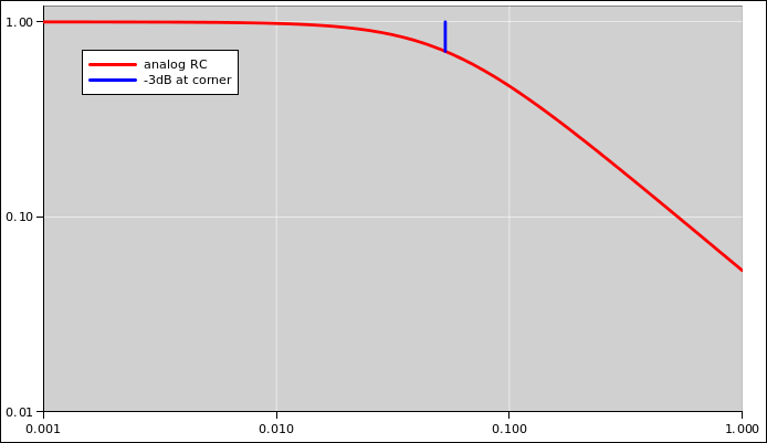
As an important application, you can find the input/output relation for the RC circuit shown in figure 1:
| (14) |
This is nothing more or less than the familiar voltage-divider formula, with the complex impedances plugged in. You see why this is called a low-pass filter. At low frequencies, it has a gain of 1. At high frequencies, the output is 90 degrees out of phase with the input, and when plotted on log-log axes, the gain falls off with a slope of 6 dB per octave, i.e. a factor of 2 in voltage for every factor of 2 in frequency, as shown by the dotted line in figure 3.
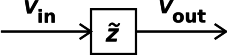
Now suppose we have a delay line that delays all signals uniformly, delaying them by a time τ, as indicated in figure 2
It is easy to show, starting from equation 3, that the voltage at the output is related to the voltage at the input by the simple relation:
| (15) |
where we define
| (16) |
Note that a factor of z makes the signal earlier, while z−1 makes the signal later. This famous “z transform” is named for this z. Note that the so-called z transform is not really a transform at all. It is just a collection of techniques that revolve around z and various powers of z, where z−1 is the phasor representation of a delay.
Let’s start with the familiar expression for Ohm’s law:
| (17) |
For linear AC circuits, we generalize this to
| (18) |
where Z represent the complex impedance. Let’s focus on the case where Z = R + 1/iωC for a resistor in series with a capacitor.
Another quantity of interest is the dissipated power:
| (19) |
The problem is, in the last two equations the symbol “V” is being used with two different, inconsistent meanings. We can clarify things by rewriting the two equations as:
| (20) |
| (21) |
The unadorned symbol V is ambiguous. It could be interpreted as V̂ or as V. Interestingly enough, equation 17 is equally valid under either interpretation. In contrast, the V in equation 18 must be interpreted as the phasor V̂ (as in equation 20, whereas the V in equation 19 must be interpreted as the real voltage V (as in equation 21). Because equation 19 is nonlinear, the phasor interpretation would be quite wrong. If you have a phasor, you simply must convert it to a real voltage before calculating the power. Otherwise you will get things spectacularly wrong.
For example, consider a wave with sine-like phase (as opposed to cosine-like phase). It is represented by a pure imaginary phasor. If you incautiously plug that into equation 19 and turn the crank, you will calculate a negative power, which is about as wrong as it possibly could be.
Notation that is convenient in one context is not always convenient in other contexts. Tradeoffs must be made. For example:
Suggestion: When you write, it is often helpful to include a legend or glossary, explaining what terminology you are using and what you mean by it. This applies to writing software as well as writing prose.
Example:
| (22) |
Some additional suggestions and caveats:
As for the term phase, sometimes it refers to the total phase
| (23) |
and sometimes it just refers to the initial phase φ0. I’m not going to argue that one is more correct than the other; they’re just different. To help reduce the ambiguity, it is a good habit to write a subscript 0 on φ0, and to use the word total when referring to the total phase.
As for the term frequency, if the frequency is constant then equation 23 is just fine. However, if the frequency is changing, for instance in the context of FM (frequency modulation), then we must consider the instantaneous frequency ω(t). The total phase becomes
| (24) |
Let’s be clear: If you naively write the phase as φ(t) = ωt + φ0 and then change the frequency, you will get wildly wrong answers.
As for the term amplitude, sometimes it refers to the A that appears in equation 5, in which case it could be positive or negative. Alternatively, sometimes amplitude refers to |A|. Another possibility is the RMS amplitude, which is about 30% smaller:
| (25) |
Sometimes instead of talking about the amplitude people talk about the peak-to-peak swing, i.e. 2|A|.
Quite often, people indicate what notion of amplitude they are using by putting subscripts on the units of measurement (rather than on the thing being measured). This is not the least bit logical, but it is so common that you might as well learn to tolerate it. Here are three equivalent ways of describing the same waveform:
| (26) |
The far more logical approach is to attach the “RMS” to the thing being measured (as in equation 25), rather than to the unit of measurement (as in equation 26). According to the SI system of units, there is no such thing as an “RMS” volt (Vrms) or a “peak-to-peak” volt (Vp-p) ... there is only the plain old volt (V).