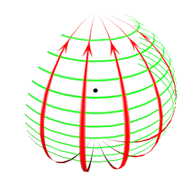
Figure 1: The 1/kr Term for a Spherical Wave
Assuming:
then:
| (1) |
where:
| (2) |
Reference: Jackson equation 9.18.
Jackson derives the equation in Cartesian coordinates, but it can equally well be interpreted in terms of spherical polar coordinates.
The first line of equation 1 is purely transverse. The other lines are not.
In the limit of small r or small k, only the last line in equation 1 survives. This is the familiar electrostatic dipole.
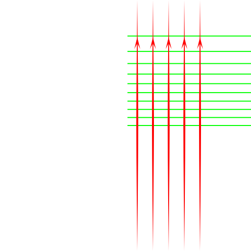
In the limit of large r or large k (but assuming the source is still tiny compared to 1/k), only the first line of equation 1 survives. This is the familiar “far field” radiation pattern.
There are two limits (near and far), but there are three terms, so you cannot think of the overall field as simply the near-field term plus the far-field term. In particular, the electrostatic dipole term falls off like (1/kr)3 but the middle term falls off more slowly, namely (1/kr)2. Let’s be clear: In the not-very-far-field zone, the dominant correction term goes like (1/kr)2, not (1/kr)3.
Perhaps more importantly, it’s better to think of it on a term-by-term basis — rather than a zone-by-zone basis. There is a rigorous distinction between the three terms in equation 1, but there is no sharp boundary between the near-field "zone" and the far-field "zone".
FWIW Jackson defines three zones: The near-field zone, the intermediate zone, and the far-field zone. Sometimes he refers to the intermediate zone as the "induction" zone, whatever that means. Still, though, it is better to focus on the terms (rather than the "zones") — the (1/kr) term, the (1/kr)2 term, and the (1/kr)3 term.
The various terms differ only by algebraic factors of kr, not by any exponentially-large factors. It could be argued that there is no “zone” where you have purely transverse spherical waves, since by the time you get far enough away that the wave is purely transverse, it’s locally indistinguishable from a plane wave, for all practical purposes.
The near field deserves more respect than it sometimes gets. For example, near-field optical microscopy (NSOM) puts the near-field terms to good use.
As an even more familiar example, if you play music in a small room, the near-field terms for the bass notes are significant everywhere in the room. If you are listening to music via headphones, the near-field terms are significant at all frequencies.
Even if you think the near-field term is not "radiation" it’s still a wave. Nobody thinks that low-frequency sound waves are not waves.
In figure 1, the center of the sphere is shown by a black dot. Imagine a tiny dipole antenna there.
The B-field lines are shown in green. I show only two octants of these lines. I show 10 semicircles out of a possible 19 circles. The lowest visible semicircle follows the equator. Note that the density of B field lines is largest near the equator and goes to zero at the poles.
The E-field lines are shown in red. I show only two octants of the lines (a different two octants). That is, I show only 5 out of 16 equally-spaced lines. Otherwise the diagram would be too cluttered.
In reality, a field line cannot change strength. E-field lines cannot just peter out; they cannot end except on a charge. What’s really happening is that some of the lines are escaping into the third dimension, away from the surface of the sphere.
The strength of the E-field is indicated by the width of the red line. It is also indicated by the density of B-field lines. For this term in the field, E is always locally proportional to B. (Not coincidentally, the same is true for a running plane wave.) For a simple dipole radiation pattern as shown here, the field strength is proportional to the cosine of the latitude. It’s ridiculously easy to verify all these assertions. Just write the divergence operator in spherical polar coordinates.
http://isites.harvard.edu/fs/docs/icb.topic970148.files/Spherical_coord.pdf
This is one of those things that is easier to verify than to figure out ab initio.
The B-field lines in figure 1 are quantitatively correct (in contrast to the E-field lines, which are partly the proverbial artist’s impression). It’s amusing that the B-field lines are equally spaced in the z-direction (not equally spaced in latitude).
If you download the following program you can rotate the diagram in 3D: https://www.av8n.com/physics/spherical-field-lines.py which requires: https://www.av8n.com/physics/spherical-field.png
It’s probably straightforward to make the program run in a browser window, platform-independently, but that’s requires more fussing than I feel like doing right now.