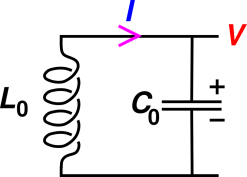
Figure 1: Energy vs Temperature for a Harmonic Oscillator
In figure 1, the dark solid curve shows the average energy of a harmonic oscillator in thermal equilibrium, as a function of temperature. (The magenta dashed line is merely a reference line, to clarify the asymptotic behavior.)
It is important to understand harmonic oscillators, because many of the things we see around us can be modeled as harmonic oscillators or collections of harmonic oscillators. For example, the heat capacity of a solid object at ordinary temperatures is well described as a collection of harmonic oscillators, one for each phonon mode.
In the figure we are measuring energy in units of ℏω, and measuring temperature in the same units. As usual, ω is the angular frequency of the oscillator, and ℏ is Planck’s constant divided by 2π.
We can learn a lot from this figure. We start by considering the limiting cases. At high temperatures, the energy of the harmonic oscillator is kT, which is the classical result, as expected. Meanwhile, at low temperatures, the energy is asymptotically ½ℏω, which is the celebrated “zero-point” energy associated with “quantum fluctuations”.
We can see that there is no difference in principle between “quantum fluctuations” and “thermal fluctuations”. This is particularly obvious in the region near the knee in the curve. The “quantum regime” is just a name we give to a particular limiting case, and the “classical regime” is just a name for another limiting case. In the general case all we can say is that there are fluctuations; we cannot say whether they are quantum fluctuations or thermal fluctuations.
Figure 1 is not some hand-wavy artist’s conception. It was computed to high accuracy based on equation 25, which is derived below.
These results help clarify an otherwise-obscure point about thermodynamic states: When thermodynamics speaks of microstates, it means quantum states. Any other notion of “microstate” would give the wrong entropy either in the high-temperature limit or the low-temperature limit. Purely classical thermodynamic arguments (such as the Gibbs Gedankenexperiment) will tell you that microstates must exist, but won’t give you a lower bound on how small a microstate can be. You need quantum statistical mechanics to do that. For the next level of detail on this, see reference 1. For the analysis of classical thermal noise in an RLC oscillator circuit, see reference 2.
By the way, it is tempting to think that ½ℏω closely corresponds to ½kT, but that’s just not right. It pays to think clearly about the following contrast:
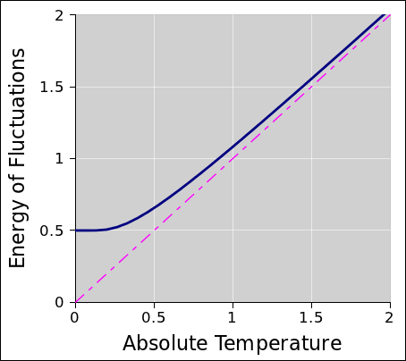
In an LC oscillator, as shown in figure 2, we must count the capacitor as one degree of freedom and the inductor as another. That makes two degrees of freedom.
In a mechanical oscillator, you can think of it as ½kT for the average thermal kinetic energy plus another ½kT for the average thermal potential energy. That makes a total of two halves kT per oscillator.
Consider the circuit shown in figure 2. This is a harmonic oscillator, consisting of an inductor L0 and a capacitor C0.
To analyze this circuit, we choose as our fundamental variable Q, the charge on the upper capacitor plate. There is a corresponding charge of −Q on the lower capacitor plate.
According to the basic capacitor law we can infer that the voltage across the capacitor is
| V := Q/C0 (1) |
By conservation of charge we can infer that the current I shown on the diagram is
| I := Q• (2) |
where the dot indicates a time-derivative.
Of particular interest is the classical energy stored in the capacitor,
| EQ := ½ |
| (3) |
and in the inductor
| EL := ½ (Q•)2 L0 (4) |
Therefore the Lagrangian can be written as
| L := ½ (Q•)2 L0 − ½ |
| (5) |
where everything is expressed in terms of the chosen coordinate Q (and its derivatives), parameterized by the component values. The first term on the RHS is a “kinetic” term, depending on the time-derivative of Q, while the second term is a “potential” term, depending on plain old Q. All this is profoundly analogous to the Lagrangian for a mechanical oscillator, such as a mass on a spring, which has the same kinetic and potential terms.
The Lagrangian L is not to be confused with the inductance L0.
Following the established principles of classical mechanics, there will be some momentum variable that is canonically conjugate to the coordinate Q, which we can calculate from the Lagrangian in the usual way:
| (6) |
We recognize I L0 as the flux in the capacitor. We denote the flux by
| φ := I L0 (7) |
We have just shown that φ is canonically conjugate to Q. That is, flux is conjugate to charge. Using these variables we can re-express the Lagrangian as
| L = ½ |
| − ½ |
| (8) |
which looks more symmetric than equation 5, and hints at the deep symmetry connecting the two mutually-conjugate variables. (We could in fact re-do the entire analysis, choosing flux as our primary coordinate. We would then re-discover that charge is conjugate to flux, and wind up with the same Lagrangian, except for an overall minus sign that has no physical significance.)
At this point we could use the principle of least action to derive the Euler-Lagrange equations and thence the classical equation of motion for the oscillator. If you do that, you find that the following is a solution for the classical equation of motion:
| Q = Q1 sin(ω t) + Q2 cos(ω t) (9) |
where Q1 and Q2 are independent of time and are called the phasor components of Q. Also we have denoted the angular frequency by ω, where
| ω := √ |
| (10) |
Classical mechanics also gives us a general expression for the Hamiltonian in terms of the Lagrangian, namely
| (11) |
Applying that to our example, we have
| (12) |
Note that starting from a Lagrangian and a chosen coordinate you can derive everything else, including the Hamiltonian, whereas starting from a Hamiltonian and a coordinate it is not possible to derive everything you need, because the Hamiltonian will not tell you what quantity is dynamically conjugate to the chosen coordinate. That is, there is no equation corresponding to equation 6 that uses the Hamiltonian instead of the Lagrangian.
Some rather fundamental principles of quantum mechanics tell us that the classical Lagrangian in equation 8 will also give us the quantum mechanical equations of motion.
In particular, recall that we ascertained via equation 6 that the classical variables Q and φ are dynamically conjugate in the classical sense.
To do quantum mechanics, we consider Q and φ to be operators. Whenever two operators are dynamically conjugate, there will be a commutation relation:
| [Q, φ] = i ℏ (13) |
Using a certain amount of hindsight we anticipate that the following operators (called ladder operators) will be useful
| (14) |
where a† is called the creation operator and a is called the annihilation operator, for reasons that will become clear shortly. Note that whereas Q and φ are Hermitian operators, neither a† nor a is Hermitian.
As a consequence of the foregoing, it is straightforward to verify the commutation relation
| [a, a†] = 1 (15) |
which can be seen as some sort of “dimensionless” version of equation 13.
It is easy to verify that the Hamiltonian operator can be re-expressed as
| H = ℏ ω (a†a + ½) (16) |
Using this and the commutation relation equation 15, it is easy to construct all the possible states, one by one. That is, suppose we are given a wavefunction |∈1⟩ that is a state of definite energy, i.e. an energy eigenstate, i.e. a state that satisfies equation 17
| H |∈1⟩ = Ê1 |∈1⟩ (17) |
Here we use a hat on Ê to remind us that Ê is the energy of a given quantum-mechanical microstate, in contrast to the energy E of a thermodynamic macrostate. This will become important later, in equation 25
So, given an energy eigenstate with energy Ê1, we can use the creation operator a† to construct another wavefunction which will also also be an energy eigenstate, with a slightly higher eigenvalue:
| H( |
| ) = (Ê1+ℏω) ( |
| ) (18) |
where the dots in the denominator stand for a normalization factor that is not of interest at the moment.
In a similar fashion, but subject to one important restriction, we can use the annihilation operator to create a wavefunction with a slightly lower eigenvalue:
| H( |
| ) = (Ê1−ℏω) ( |
| ) (19) |
It turns out that all energy eigenstates can be constructed in this way. That is, there is a lowest-energy state |∈0⟩ which satisfies the eigenvalue equation
| H |∈0⟩ = (0 + ½) |∈0⟩ (20) |
and all energy eigenstates satisfy the equation
| H |∈N⟩ = (N + ½) |∈N⟩ (21) |
for some non-negative integer N. If the oscillator is in a state of definite energy, then it has a definite integer value for N, and we say N is the number of quanta in the oscillator. Accordingly a†a is called the number operator.
To see why negative N-values are not possible in equation 21, let’s attempt to form the state a |∈0⟩, which we might imagine would have N=−1 in accordance with equation 19. But let’s look at the normalization. Consider the expression
| (22) |
The LHS can be interpreted in two ways. It could be the number operator a†a evaluated in the ground state |∈0⟩, as shown on the second line of equation 22. This makes sense, and gives zero as expressed on the RHS. Alternatively, the LHS could be simply the inner product of the state a|∈0⟩ with itself, as shown on the third line of equation 22. That’s a problem, because the inner product of any state with itself should be 1, since the state vectors are normalized. We have a proof by contradiction: If the N=−1 state existed, it would be normalized, but since it can’t be normalized, it must not exist. And since this state cannot be constructed, yet-lower states with N<−1 cannot be constructed either.
To summarize, if we assume that |∈0⟩ exists, we can construct all |∈N⟩ for non-negative integer N. We have proved that negative integers are not allowed. We have not bothered to prove that |∈0⟩ exists, and we have not proved the impossibility of non-integer quantum numbers; doing that would require actually solving the equation of motion to find the wavefunctions. It is remarkable how much we have been able to do just from the commutation relations, without ever touching the equation of motion.
If you want to see what some of the wavefunctions look like, see e.g. reference 3.
We can use the energy eigenstates as a basis for the whole state space. This allows us to enumerate all the states, and we know the energy for each one. The energy of the Nth energy eigenstate is (N+½)ℏω.
Therefore the partition function is:
| (23) |
where as usual, β denotes the inverse temperature, β := 1/kT.
The sum on the second line of equation 23 is a geometric series, and can be summed using the usual trick. That gives us
| (24) |
It is remarkable that the partition function is expressible in such a simple closed form.
We can now use the familiar machinery of statistical mechanics to find quantities of interest, such as the average energy:
| (25) |
We can gain some insight into this result by considering the limiting cases. When β is small, i.e. at high temperatures, the coth is well approximated by the inverse of its argument, so the energy is just 1/β. That is, at high temperatures, the energy of the harmonic oscillator is kT, which agrees with the classical result, as expected in accordance with the correspondence principle. Meanwhile, when β is large, i.e. at low temperatures, the coth goes asymptotically to 1, and the energy is just ½ℏω, which is the celebrated “zero-point” energy.
Figure 1 is a graph of this function, showing both limiting cases.