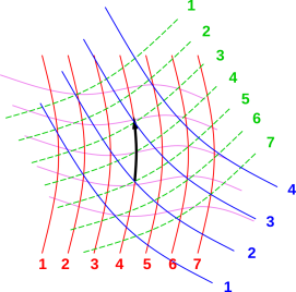
Figure 1: Contours of Constant R, G, B, and V
Executive summary: Partial derivatives have many important uses in math and science. We shall see that a partial derivative is not much more or less than a particular sort of directional derivative. The only trick is to have a reliable way of specifying directions ... so most of this note is concerned with formalizing the idea of direction. This results in a nice graphical representation of what “partial derivative” means. Perhaps even more importantly, the diagrams go hand-in-hand with a nice-looking exact formula in terms of wedge products.
Partial derivatives are particularly confusing in non-Cartesian coordinate systems, such as are commonly encountered in thermodynamics. See reference 1 for a discussion of the laws of thermodynamics.
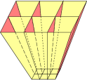
We will illustrate the discussion with a sample problem. Let there be five variables, namely {R, G, B, V, and Y}, four of which are explicitly shown in figure 1. Let there be D degrees of freedom, so that these five variables exist in an abstract D-dimensional space. We assume that the number of variables is larger than D, so that not all of the variables are independent. The relationships among the variables are implicit in figure 1. We will use the information in the figure to find the partial derivatives, and then the partial derivatives can be integrated to find the explicit relationships.
For simplicity, you can focus on the D=3 case, but the generalization to more degrees of freedom, or fewer, is straightforward, and will be pointed out from time to time. (Remember that D has nothing to do with the dimensionality of the physical space we live in.)
In accordance with an unhelpful thermodynamic tradition, you may be tempted to identify D of our variables as “the” independent variables and the rest of them as “the” dependent variables. Well, do so if you must, but please bear in mind that the choice of independent variables is not carved in stone. My choice may differ from your choice, and for that matter I reserve the right to change my mind in the course of the calculation. As discussed at length in section 2 and section 5, we can get along just fine treating all variables on an equal footing.
Also note that having only five variables is a simplification. In a real thermodynamics problem, you could easily have ten or more, for instance energy, entropy, temperature, pressure, volume, number of particles, chemical potential, enthalpy, free energy, free enthalpy, et cetera. There could easily be more, especially if you have D>3 degrees of freedom.
The point is, variables are variables. At each point in the abstract D-dimensional space, each of our variables takes on a definite value. In the jargon of thermodynamics, one might say that each of our variables is a “thermodynamic potential” or equivalently a “function of state”. Trying to classify some of them as “dependent” or “independent” requires us to know more than we need to know ... it requires us to make decisions that didn’t need to be made.
We will be using vectors, but we will not assume that we have a dot product. (This situation is typical in thermodynamics.) As a result, there is no unique R direction, G direction, B direction, V direction, or Y direction. The best we can do is to identify contours of constant R, G, B, V, and/or Y. In figure 1,
It is worth re-emphasizing: There is no such thing as an R axis in figure 1. If there were an R axis, it would be perpendicular to the red curves (the contours of constant R), but in this space we have no notion of perpendicular. We have no notion of angle at all (other than zero angle), because we have no dot product. The best we can do is to identify the contours of constant R. Any step – any step – that does not follow such a contour brings an increase or decrease in R. There are innumerably many ways of taking such a step, and we have no basis for choosing which direction should represent “the” unique direction of increasing R.
| You can’t specify a direction in terms of any one variable, because almost every variable is changing in almost every direction. If we had a dot product, we could identify the steepest direction, but we don’t so we can’t. | The best way to specify a direction is as the direction in which a certain D−1 variables are not changing. This works always, with or without a dot product. |
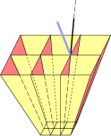
In our sample problem, D=3. The black arrow in figure 1 represents a direction, namely the direction of constant R and constant Y.
In general, it is unacceptable to think of ∂G/∂B as being the derivative of G with respect to B “other things being equal” – because in general other things cannot be equal. Which other things do you mean, anyway? Constant R? Constant V? Constant Y?
Sometimes, the context might indicate which other things are to be held constant – but if you rely on this, it’s just a matter of time before you get into trouble. If there is any doubt, rely on the idea of directional derivative, and specify the direction. So a proper partial derivative can be written as:
| ⎪ ⎪ ⎪ ⎪ |
| (1) |
which is pronounced “the partial derivative of G with respect to
B at constant R and Y”.
The black arrow in figure 1 depicts the physical meaning of equation 1. To evaluate the derivative, take an infinitesimal step in the direction of constant R and Y, as shown by the arrow. The length of the step doesn’t matter, so long as it is small enough; the length will drop out of the calculation.
Next, count the number of G-contours crossed by the vector. This will be the numerator. In our sample problem, the numerator is 2. Also count the number of B contours crossed by the vector. This will be the denominator. In our sample problem, the denominator is 1. Then divide numerator by denominator. We conclude that
| ⎪ ⎪ ⎪ ⎪ |
| = 2 (2) |
We take this as the definition of partial derivative: take a step in the given direction. This gives us two points in space, the tip-point and the tail-point. There will be a difference in the “numerator” variable (tip minus tail) and a difference in the “denominator” variable (tip minus tail). Divide the differences, and take the limit as stepsize goes to zero. That’s it.
By the way, when most people see diagrams such as figure 1, they are tempted to call it the “geometric interpretation” of a partial derivative. Technically, though, that’s not the right name, because if you don’t have a metric, you don’t have a geometry. Properly speaking, what we are doing here is differential topology, not geometry. Of course, if you wish to conjure up a metric, you can re-interpret everything in terms of geometry ... but the discussion here is quite a bit more general than that. In particular, all the relationships discussed here are invariant if you stretch the paper on which the diagrams are drawn. That’s the hallmark of topology, setting it apart from geometry.
Let dG be the exterior derivative of G. We can expand this in various ways, including
| dG = |
| ⎪ ⎪ ⎪ ⎪ |
| dB + |
| ⎪ ⎪ ⎪ ⎪ |
| dR + |
| ⎪ ⎪ ⎪ ⎪ |
| dY (3) |
Since there are D degrees of freedom, there will be D terms on the
RHS. That is, any complete expansion will expand dG in terms of
D linearly-independent one-forms (in the general case, i.e. with
only trivial exceptions). (We shall have more to say about the
physical significance of this expansion in section 5. See
reference 2 for the basic properties of
differential forms. See reference 3 for how they apply
to thermodynamics.)
The interesting thing is that you can choose any three variables as a basis, so long as they are linearly independent, i.e. dB∧dR∧dY ≠ 0. For example, instead of using {B, R, Y}, we can equally well expand G in terms of {V, R, Y}, as follows:
| dG = |
| ⎪ ⎪ ⎪ ⎪ |
| dV + |
| ⎪ ⎪ ⎪ ⎪ |
| dR + |
| ⎪ ⎪ ⎪ ⎪ |
| dY (4) |
There is no requirement that the basis one-forms be orthonormal
... and indeed we don’t even have any notion of orthogonality or
normalization, because we don’t have a dot product. The rule is
simple: in each term, you differentiate with respect to one variable
while holding constant the other D−1 variables in your basis-set.
This section should make it clear that we are not required to express G as a function of B, R, and Y. That is allowed, but not required. Every point in this space has its own value of G, B, R, V, Y, and other variables besides. Given any three of these variables, you can determine all of the others (at least locally, assuming linear independence).
This is worth emphasizing, because there are some thermodynamics books that might leave you with the impression that energy exists only its own special space where volume and entropy are “the” independent variables, while the free enthalpy (i.e. Gibbs function or Gibbs potential) exists in another special space where pressure and temperature are “the” independent variables. The disadvantages of such an approach greatly outweigh the advantages.
Even if the textbook expresses the free enthalpy as a function of P and T, you are allowed to re-express it as a function of V and S, or whatever variables you choose, provided they are linearly independent. Choosing new variables is sometimes very useful, as we shall see in section 5.
In particular, returning to our abstract color-coded variables, we can have:
| (5) |
where f1, f2, etc. are functions, as the word function is understood in mathematics (you give me the abscissa and I’ll give you the ordinate), and as the word is understood in computer science (you give me the arguments and I’ll give you the return-value). It is OK to ask for the partial derivative of f1 with respect to R, because that means to hold constant the other arguments to f1. In contrast, it is risky to ask for the partial derivative of G with respect to R, because your readers might not know whether you intended to hold B constant (as on the first line of equation 5) or hold V constant (as on the second line of equation 5).
I gave the functions nondescriptive names, f1() and f2(). It would make at least as much sense to call them Gbry() and Gvry() respectively. The point here is that these names should not be abbreviated to something cute like f() or G(), because that would produce multiple ambiguities or inconsistencies. If, for instance, you write a computer program to evaluate
| G = G(7, 13, 2.2) [deprecated; too cute] (6) |
you’ll have a big mess deciding what G really stands for; possibilities include:
Some thermodynamics books use this sort of cute terminology and try to remove the ambiguities using so-called conventions. For instance, according to convention, the energy E is “naturally” a function of the volume V and the entropy S. Such conventions sometimes suffice for working the baby problems at the end of the chapter, but as soon as you try to work real industrial-strength problems, things go to pot. For starters, cute notation leads to misconceptions and bad habits. What’s worse, the conventions are simultaneously too strict and too loose. The conventions prevent you from writing things that you might have good reason to write (as we shall see in section 5), yet there are not enough conventions to remove all the ambiguities.
Consider the comparison:
| When dealing with pointy vectors, we think of a vector X as having one-dimensional extent. We visualize its magnitude as being a length. | When dealing with one-forms, they are vectors in accordance with the axioms that define what a vector space is ... but they are different from pointy vectors. We visualize the one-form dG in terms of shells of constant G. Each shell has codimension 1, i.e. it has dimension D−1. In our three-dimensional example, the shells are surfaces. We visualize the magnitude of the one-form as how closely-spaced the surfaces are. |
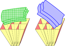
| We think of a bivector X∧Y as having two-dimensional extent. We visualize its magnitude as the area of a parallelogram. | A two-form such as dG∧dR can be represented as a bunch of lines, like flux lines. The magnitude of the two-form is given by the number of lines poking through a given area. (It has nothing to do with the length of the lines, and it is inversely related to the lateral spacing between the lines.) Even better, we can visualize the two-form as a bunch of tubes, as in figure 2. The magnitude of the two-form is given by the number of tubes crossing a given area. (It is inversely related to the cross-sectional area of each tube.) The aforementioned flux lines correspond to the corners where one tube meets another. |
| Similarly, the trivector X∧Y∧Y has three-dimensional extent. We visualize its magnitude as the volume of a parallelepiped. | A three-form can be represented by a bunch of cells, stacked the way sugar cubes are stacked in a large box. The magnitude of the three-form is given by the number of cells per unit volume. (It is inversely related to the volume of each cell.) |
It should be clear from the foregoing that although both bivectors and one-forms (in D=3) are in some sense surface-like, they do not behave the same. In one case magnitude is area in the surface, while in the other case the magnitude is the closeness between surfaces. Area is not the same as inverse length.
Now let’s progress from one-forms to two-forms. A familiar example of a two-form is a bundle of magnetic field lines. You can sketch them based on theory, or if you really want to visualize them, get a bar magnet and decorate the field lines using iron filings. The strength of the field is represented by the closeness of the lines, i.e. an inverse area, i.e. the number of field lines crossing a unit area.
It is visually different but mathematically equivalent to visualize a two-form as a bunch of tubes. Each tube of dR∧dY is boxed in on two opposite sides by two shells of constant R (with two successive values of the constant), and on the other two opposite sides by two shells of constant Y (again with two successive values of the constant). This is illustrated in figure 2. The magnitude of the 2-form is the number of tubes crossing a given area. The lines mentioned in the previous paragraph are just the corners of the tubes. You can count lines or count tubes, and it comes to the same thing either way.
Mathematically, an N-form is (by definition) a linear function that takes N pointy vectors as inputs and produces a scalar, and is antisymmetric under interchange of its arguments.
This allows us to establish a correspondence between (D−1)-forms and directions. Given a (D−1)-form, there is a unique corresponding direction. Specifically, we consider the (D−1)-form as an operator, and the corresponding direction is identified as a vector (a pointy vector) in the null space of the operator.
In our sample problem, the black vector, representing the direction of constant R and constant Y, lies in the null space of the 2-form dR∧dY. Figure 3 shows a perspective view of the same situation. The black vector is in the null space of the 2-form, while the blue vector is not.
Diagrammatically and physically, here’s how it works. Call the black vector X. You can create a little patch of area by forming the wedge product of X and some other vector Y. The point is that no matter what Y is, with this particular X, the area X∧Y is not crossed by any tubes of the two-form dR∧dY.
Note that we were able to establish this correspondence between a (D−1)-form (dR∧dY) and a vector (X) without using a metric, i.e. without any notion of dot product, angle, or length.
Also, to be explicit: I’ve been using the term “direction” to denote an equivalence class of pointy vectors, each of the which can be computed from another by multiplying by a nonzero scalar. (If we were given a dot product, we could have used the simpler notion of a unit vector in the given direction, but since we don’t have a dot product we have no notion of “unit” vector, so we use the equivalence class instead.)
As nice as this direction vector is, in the next section we shall construct something even nicer.
In the previous section, the “direction vector” was defined as being in the null space of a (D−1)-form. The problem is, even if you have a clear pictorial and conceptual understanding of what that vector is, I haven’t given you any algorithm for actually calculating that vector.
And it turns out we don’t need to calculate that vector, because there is something better, conceptually as well as computationally. We don’t much care about the null space of dR∧dY anyway; what we really care about is the non-null space.
So let’s cut to the chase. The partial derivative can be expressed as:
| ⎪ ⎪ ⎪ ⎪ |
| = |
| (7) |
and the physical significance of this is depicted in figure 4:
The contours of constant B are shown in blue, and similarly for the other variables: G (hatched green), Y (yellow), and R (red).
The numerator in equation 7 is a 3-form, so we visualize it as a bunch of cells; the magnitude of the 3-form is given by the number of cells per unit volume. The same goes for the denominator.
The numerator has D−1 factors that it shares with the denominator, plus one unshared factor.
In figure 4, compared to the blue contours, the green contours are both more closely spaced and better aligned, so the partial derivative ∂G/∂B |R,Y is greater than one.
Also: The correctness of equation 7 can be proved by expanding dG according to equation 3 and plugging that into equation 7. All the terms except the one you are interested in vanish, because they involve things like dR∧dR, which is manifestly zero.
Let us discuss the usefulness of expressing partial derivatives in terms of spatial relationships and differential topology, as presented above.
One argument is that the form of equation 7 is well-nigh unforgettable, and provides a clear recipe for calculating the desired partial derivative.
Another argument argument stems from the fact that the RHS of equation 7 uses the variables that vary during the differentiation (G and B) on essentially the same footing as the variables held constant (R and Y) – as factors in a wedge product. This stands in stark contrast to the LHS, where differentiating looks irreconcilably different from holding-constant. I find the even-footed version vastly more elegant. It is also quite practical, as illustrated by the following example.
To say the same thing more concisely: The structure of equation 7 tells us things that might otherwise be non-obvious, as we now discuss.
Let’s do an example involving real thermodynamic variables. Following the model of equation 3, let’s expand the energy (E) in terms of the entropy (S), the volume (V), and the number of particles (N).
| dE = |
| ⎪ ⎪ ⎪ ⎪ |
| dS + |
| ⎪ ⎪ ⎪ ⎪ |
| dV + |
| ⎪ ⎪ ⎪ ⎪ |
| dN (8) |
As an aside, we note that the partial derivatives in this expansion have conventional names, namely the temperature, negative pressure, and chemical potential; specifically:
T :=
∂E ∂S ⎪
⎪
⎪
⎪
V,N −P :=
∂E ∂V ⎪
⎪
⎪
⎪
N,S µ :=
∂E ∂N ⎪
⎪
⎪
⎪
S,V (9)
whence
dE = T dS − P dV + µ dN (10)
Returning to the main line of argument, let’s re-express equation 8, writing the partial derivatives in terms of wedge products, i.e. in terms of counting cells in space:
| dE = |
| dS + |
| dV + |
| dN (11) |
where I have used the anticommutative property of the wedge product to write the fractions in a more suggestive form. We see that the partial derivatives share a common denominator. (This is a property of all such expansions.)
This common denominator suggests a few games we can play, such as dividing one partial derivative by another:
| (12) |
where the last step uses the anticommutativity of the wedge product. Translating equation 12 into the conventional notation for partial derivatives, we get
| (13) |
whence
| = |
| ⎪ ⎪ ⎪ ⎪ |
| (14) |
Let’s discuss this for a moment. There is a whole family of
identities that you can construct using the same basic technique. I
don’t know what to call them. They’re not Maxwell relations; a
Maxwell relation is an identity involving second derivatives,
exploiting the equality of the mixed partials. In contrast,
equation 13 involves only first derivatives. The topological
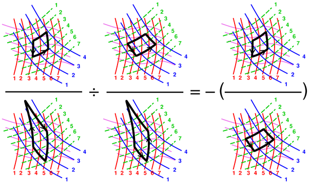
interpretation of such an identity is shown in figure 5.
Remember that the magnitude of a 2-form is always given by the number of cells per unit area, so in figure 5 each magnitude is inversely related to the size of the black-outlined area.
Figure 5 is a very direct portrayal of the following identity in D=2, i.e. in the plane of the paper
| ÷ |
| = − |
| (15) |
and if you imagine another degree of freedom, the same figure portrays
the following identity in D=3
| ÷ |
| = − |
| (16) |
where the contours of constant Y are not visible because they run parallel to the plane of the paper.
Actually I find it easier to visualize what’s going on by looking at equation 16 than by looking at figure 5. When I look at the equation, I “see” little cells in space.
In particular, keep in mind that a differential form has a direction of circulation associated with it.
| The two denominators on the LHS in figure 5 have the same magnitude and the same shape, but if you look closely you see that they have opposite circulation, and that’s why there is an explicit minus sign on the RHS of the figure. | In expressions such as equation 16, to keep track of the sign of the differential form, it is necessary and sufficient to keep track of the ordering of the factors in the wedge products. This is easier than making a diagram detailed enough to keep track of the direction of circulation. |
These identities nicely demonstrate the usefulness of the wedge-product approach. Suppose somebody asks you to verify the validity of equation 14. You could attack it using conventional calculus techniques, but that would be markedly messier than the approach presented here.
What’s worse, the conventional method of calculation provides little insight, so that you are left wondering how anybody could possibly have discovered equation 14. If you ever forget the result, you’ll have a hard time re-discovering it, unless you have tremendous insight ... or unless you express the partial derivatives in terms of wedge products.
Also note that the RHS of equation 14 is a classic example of writing non-conventional ordinates in terms of non-conventional abscissas, as foreshadowed in section 2. Specifically, the physical significance of this equation is as follows: Suppose we start with some gas in an isolated vessel of volume V, and we know the values of E, P, S, T, N, et cetera. Next we open a valve connecting to a small evacuated side-chamber, so that the gas undergoes free expansion into a slightly larger volume. Then equation 14 tells us how the entropy changes.
Let us briefly restrict attention to ideal gases. (The rest of the discussion is free of such restrictions.) Using the ideal-gas law, PV = NkT, we can rewrite equation 14 as
| = |
| ⎪ ⎪ ⎪ ⎪ |
| (17) |
If we move the ∂V to the LHS,
we can integrate both sides (along a path of constant E and
constant N). This yields the well-known result that under
conditions of free expansion, the entropy of an ideal gas is a
logarithmic function of the volume:
| S = Nk ln(V) + const (18) |
Joule-Thompson expansion is another example – an example with
historical and practical significance – involving expansion at
constant E and constant N.
Equation 14 is a genuine, non-trivial result, obtained with remarkably little work.