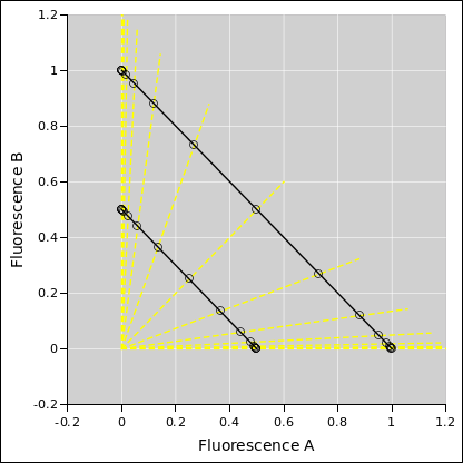
Figure 1: Fluorescence Curves Separately
This document makes a tremendous number of idealizations and simplifications. That’s a polite way of saying the details are mostly wrong. However the details are fixable, and the basic idea probably stays the same, even if the details change.
We have a fluorescent dye molecule. It has a protonated form and a non-protonated form. The two forms fluoresce at different wavelengths. So by measuring the two fluorescence signals we are basically measuring the population of the two forms. The idealized dependence is shown in figure 1.
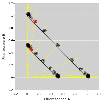
Temporarily, imagine the pH is given and we want to predict what the fluorescence data will look like. Let’s replot the data from figure 1 on different axes, namely A versus B axes. That corresponds to the upper curve in figure 2. The lower curve corresponds to the same data, but the overall intensity is scaled by a factor of 0.5, which is what we get if the dye concentration is lower and/or the dye is not in the optimally sensitive region of the optical apparatus. In this ideal (A, B) space, the yellow tie-lines are contours of constant pH. Each tie-line differs from the next by half a pH unit, increasing from upper-left to lower-right. The central line (the 45∘ line) corresponds to pH 7, and you can count up or down from there. Similarly, the discrete points (shown as circles in the figure) correspond to integer and half-integer values of pH.
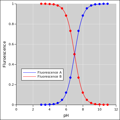
Now imagine there is some noise on the fluorescence data. For starters, let’s imagine some additive noise. In particular, the additive noise is purely positive, such as we would get from some sort of additive background. (In the real world we would also want to model Poisson noise, which is not purely additive, but let’s not worry about that at the moment.) That gives us something like figure 3:
As a point of terminology:
| (1) |
One thing to notice is that the dimensionless ratio (A−B)/(A+B) is a sufficient statistic for determining the pH in the ideal case as shown in figure 2. That is to say, if you know that ratio, you don’t need to know A or B separately. (BTW FWIW you could equally well use A/(A+B) or B/(A+B) or simply A/B as a sufficient statistic ... in the ideal noiseless case. All these quantities are related, via simple one-to-one relationships.)
However, in the presence of noise, we need to determine the error bars on the estimated pH, and alas the dimensionless ratio (A−B)/(A+B) is not a sufficient statistic for that. The uncertainty on the pH depends on the dimensionful quantity (A+B). You can see this by looking at the red points i.e. the pH 6 points in figure 3. The pH 6 data is cleanly separated from the pH 5.5 (and lower) data on the upper curve (A+B=1), but not so cleanly separated on the lower curve (A+B=0.5). The error bars on the pH are considerably longer in the latter case, but the dimensionless ratio won’t tell you that.
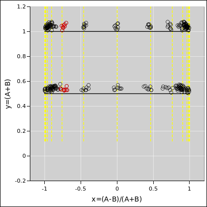
Another thing to notice is that the noise introduces a systematic bias. Because the additive noise is always positive, it shifts the observed data (A′, B′) toward the 45∘ line, shifted relative to the corresponding ideal noiseless (A, B) point. This can be seen in the ph 6 data, shown in red in figure 3 and figure 4. The points are systematically to the right of the yellow tie-line.
Some of the systematic bias could be removed via the calibration process, but it has to be done carefully. In particular, the dimensionless ratio (A−B)/(A+B) is not a sufficient statistic for determining the amount of bias.
We started by thinking of A and B as “the” parameters of the model, but it may be convenient to rotate and rescale the axes as follows:
| (2) |
That is approximately a 45∘ rotation, followed by a rescaling of the x axis. The result is shown in figure 4.
For the purposes of data analysis, we want to infer the pH, given some observed A′ and B′. This is the inverse of the problem discussed in section 1. That is, the previous given has become the output, and the previous outputs have become the givens.
We start by considering a simplified case, where only one inference is required. The more general case is discussed in section 3.
As with any inverse problem, it can be formulated as a search. In the simplified case, it suffices to search through “model parameter space” to find the parameters that best explain the observed A′ and B′. Then to calculate the error bars, we re-do the search, to find the range of parameters that is reasonably consistent with the observed A′ and B′. This search can be formulated as a search through (x, y) space, as defined in equation 2.
Searching gives us a way to calculate the maximum a priori probability that a given pH and a given intensity will produce the observations. Keep in mind that pH and intensity are parameters of the model we are using. Also the amount of noise is a parameter of the model.
| (3) |
The fact the noisy data does not fall on the ideal calibration curve is not a problem. We are searching for pH values that are consistent with the data, taking into account both the ideal calibration curve and the noise model.
By definition, the term likelihood refers to the a priori probability, namely the probability of the observations given the model. In the context of data analysis, this by itself is almost never the final answer, but it’s a step in the right direction. It is an ingredient that contributes to the right answer.
What we almost certainly want it the maximum a posteriori probability
| (4) |
In reality, we really are given the observations, and we want to infer the model parameters ... not the other way around.
We can get from equation 3 to equation 4 using the Bayes inversion formula. It must be emphasized that there are two inversions going on here; first we need to change our mind about what’s the independent variable and what’s the dependent variable. Then we need to move each variable to the proper side of the “given” bar in the expression for conditional probability.
If we have some Bayesian prior on pH-values, this is where we get to take that into account. If it is a smooth prior and/or if we have a high confidence in the data, the prior doesn’t matter much. Conversely, if it is a narrow peaky prior and the data is noisy, then the prior matters a great deal.
The previous sections assumed we could directly measure the fluorescence cross section. In fact we cannot. We have to infer the cross section from other things that are more directly measurable.
This is no big deal; it is just another inverse problem, similar to the one we have already discussed. In fact, there are layers upon layers of inference.