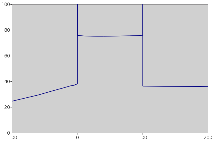
Figure 1: Water: Enthalpy versus Temperature
Figure 1 plots the molar enthalpy of water versus temperature.
Note: For simplicity, in this document we assume constant pressure. In particular, “heat capacity” is shorthand for “heat capacity at constant pressure”. For details on what we mean by enthalpy, temperature, heat capacities, et cetera, see reference 1.
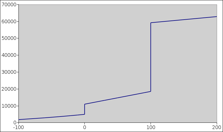
For starters, let’s take a look at the slope of this curve, and limit attention to places where the slope is well behaved. (We will deal with the ill-behaved places later.) We define slope in the usual way: The slope at a point is the “rise over run” as measured in some small neighborhood around that point. The slope of this curve is called the molar heat capacity and is denoted cP. Figure 2 plots the molar heat capacity versus temperature, subject to some limitations that we will discuss in a moment.
In both of these figures, there are two places where talking about the “slope” doesn’t tell us what we want to know. These are the places where a first-order phase transition is occurring.
For H2O at STP, the solid/liquid phase transition occurs at 0C, and the liquid/vapor phase transition occurs at 100C. Each of these is a first order phase transition.
In all generality, there is a latent heat associated with any first-order phase transition. Melting and vaporization are not the only examples; the Curie point in a ferromagnet is another important and interesting example.
The molar latent heat not a slope, because it is purely a “rise” without any associated “run”. Therefore we have two distinct concepts that we need to keep straight, namely heat capacity and latent heat. In figure 1, it is relatively easy to visualize both concepts at the same time. The following table summarizes the situation:
| name | ... | geometry | ... | SI unit |
| molar heat capacity | ... | rise over run | ... | J/K/mol |
| molar latent heat | ... | rise without run | ... | J/mol |
It is straightforward to calculate the heat-capacity-versus-temperature curve (figure 2) by finding the slope of the enthalpy-versus-temperature curve (figure 1) ... except near the phase transitions.
When creating figure 2, we have a dilemma:
In particular, let’s think about the spikes in figure 2. The spikes extend far above the top of the page. If you don’t want to consider them as absolutely infinite, you can imagine that the spike at the solid/liquid transition is (say) one millikelvin wide and 6 million J/mol high. In any case, no matter how you imagine the height and width, the area under the curve, due to this spike alone, is 6000 J/mol, i.e. the molar latent heat. Similarly the area under the spike at the liquid/vapor transition is 40,000 J/mol, which you can (optionally) approximate by drawing it 1 mK wide and 40 million J/K/mole high. In reality the spikes are even narrower and higher than that.
You can confirm that these numbers (6000 and 40,000) are the right numbers by looking at the heights of the steps in figure 1.
Let’s be clear: In figure 2 and in all similar plots, area under the spike is well defined, even though the height and width of the spike are not well defined. A spike that has this property is called a distribution.
The solid/liquid phase transition is also known as the melting point, or (equivalently) the freezing point. The liquid/vapor phase transition is also known as the boiling point, or (equivalently) the dew point. Calling such things “points” is a misnomer. The transitions are definitely not pointlike if you look at the phase diagram at a whole. The transitions cast pointlike projections on the temperature axis, but not on the other axes.
In figure 1, it would be nice to speak of the enthalpy as a “function” of temperature ... except that it is not a function! Strictly speaking, a function has only one ordinate for each abscissa, whereas there are two places where this curve has multiple ordinates for a given abscissa. In particular, the points (100,20000), (100,40000), and (100,60000) are all perfectly respectable points on the entropy-versus-temperature relationship.
The recommended conventional terminology is to call it a mapping instead of a function. We can say there is a mapping from temperature to enthalpy. It is also acceptable to say there is relationship between enthalpy and temperature. Just keep in mind that this relationship is not a function.
By the same token, the so-called “Dirac delta function” is not a function, despite the name. It is a distribution, so it really should be called the Dirac delta distribution. It has unit area under the curve and zero width. Loosely speaking, it has infinite height.
Strictly speaking, the heat capacity CP is an extensive quantity, written with a capital C. Often, especially in theoretical discussions, we are more interested in one of the corresponding intensive quantities, either the specific heat capacity (i.e. heat capacity per unit mass) or the molar heat capacity, written cP with a small c.
As discussed in reference 2, the word “heat” by itself has multiple inconsistent meanings, and arguing about “the” definition is a fool’s errand.
In this document we use the word “heat” only as part of idiomatic expressions such as “heat capacity” and “latent heat”, where the expression as a whole can be defined without reference to the definition of the individual words.
There are several options for describing the enthalpy-versus-temperature behavior of a substance.
It is good to mention the problems with the heat-capacity near a phase transition, but it is pointless to spend much time trying to solve them. Instead, it is simpler and better to focus most of the discussion on the enthalpy (as in figure 1), where both the heat capacity and latent heat can be nicely visualized.