Figure 1: Entropy of the Poisson Distribution
For any µ and ν, the joint probability that µ takes on the value a and ν takes on the value b will be denoted P(µ:x, ν:y).
The conditional probability that µ takes on the value a, given that ν takes on the value b, will be denoted P(µ:x | ν:y).
Similarly, the conditional probability that ν takes on the value b, given that µ takes on the value a, will be denoted P(ν:y | µ:x).
Note that P(µ:3 | ν:7) is a completely different concept from P(ν:3 | µ:7) ... so we can see why the conventional notation of just writing P(µ | ν) is abominable: it leads you to write things like P(3 | 7) which is hopelessly ambiguous.
The unconditional probability that µ takes on the value a is denoted P(µ:x).
Some basic identities include:
| (1) |
which pretty much defines what we mean by conditional
probability. As a corollary,
| P(ν:y | µ:x) = |
| (2) |
which is called the Bayes inversion formula.
In the case of Poisson distribution, suppose we know (based on an ensemble of measurements) that the average count in a certain time-interval is λ. Then the probability that in a given trial we observe k counts in the interval is:
| P(K:k | Λ:λ) = e−λ |
| (3) |
It is an easy and amusing exercise to verify that this formula
normalized so that
| P(K:k | Λ:λ) = 1 for any λ (4) |
as it should.
Also by way of terminology, note that the term likelihood is defined to mean the a priori probability, namely P(data | model). In the data-analysis business, maximum-likelihood methods are exceedingly common ... even though this is almost never what you want. We don’t need a formula that tells the probability of the data; we already have the data! What we want is a formula that allows us to infer the model, given the data. That is, we want a maximum-a-posteriori (MAP) estimator, based on P(model | data).
Preview: The main point of this section is that maximizing the likelihood is the same as minimizing the cross entropy, which is the same as minimizing the KL information divergence.
To see why, suppose we have a radioactive source that emits particles at a steady rate r. We observe it over a time interval with width w and count the particles. We repeat this experiment N times. Let the observed counts by ki, for all i from 1 to N.
The probability of observing a particular sequence {ki} is:
| (5) |
where the intensity λ is equal rw. Neither the rate r nor the window width w matters directly to the Poisson distribution; only their product matters. We can rewrite this as a sum:
| (6) |
We use the negative log, because P is less than one, and we prefer to deal with positive numbers. So this is an equation for the log improbability.
It is amusing to convert the sum over i to a sum over k, as follows:
| (7) |
where Mk is a multiplicity factor, keeping track of how many times a particular k value appears in the sum in equation 6. If the data is sparse, most of the Mk will be 0 and a few of them will be 1. On the other hand, if we have a huge amount of data, the Mk will converge to predictable values. In fact, Mk/N will converge to the probability of getting a particular k value. Therefore:
| (8) |
So the average log improbability per observation is just the entropy. The factor of N makes sense because entropy S is a property of the distribution, defined as an average (not a sum) over the distribution. It doesn’t care how many times you repeat the observation. In contrast, the likelihood P depends on the product (not the average) over all observations.
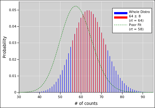
When plotted on semi-log axes, as in figure 1, the asymptotic slope is 1/2. In more detail:
| (9) |
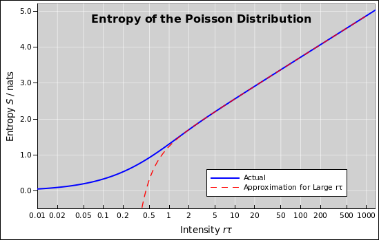
which makes sense. It is basically the log multiplicity, i.e. the log of the number of terms that contribute to the high-probability region of the probability density distribution, as shown in red in figure 2. The width of this region scales like the square root of rt (when rt is not small). When you take the logarithm, the square root becomes a factor of ½ out front.
| (10) |
where RHS is the same as before, except that the rate r in front of the logarithm is not the same as the one inside the logarithm.
Here is how we interpret this: Suppose we have some data, and we wish to fit a model to the data, in order to determine the rate r. There is some robs that is known to Mother Nature but not directly known to us, which is what controls the observations. We hypothesize a rate rmod to use in our model, and we adjust it to obtain the best fit.
We have no control over robs, so for the purpose of curve fitting we consider the cross entropy to be a function of rmod. The minimum value of the cross entropy occurs when rmode is equal to robs. You can understand this with the help of the dashed green curve in figure 2. To get the extremal value in equation 10, it would be best to have the green curve (which represents the model) line up with the blue and red histogram (which represents the observations). That makes the largest value of the logarithm line up with the largest value of the factor out front. Shifting the green curve in either direction gives more emphasis to the low probability (high improbability) parts of the curve.
If we subtract off this extremal value, we are left with something that is zero for an exact match, and positive otherwise.
| (11) |
It is tempting to think of this as measuring the “distance” between two distributions, but that is not recommended. The problem is that the genuine distance should be symmetric. That is, the distance should be the same when going from A to B as when going from B to A. The Kullback-Leibler information divergence is, alas, not symmetric.
The main point of all this is that maximizing the likelihood is the same as minimizing the cross entropy, which is the same as minimizing the KL information divergence.
By way of analogy: Suppose we have 50 readings, and we want to know the average. One analyst averages the readings directly in the obvious way. Another analyst averages them in groups of 10, and then averages the 5 groups. Both methods produce the same answer. This is a consequence of the fact that averaging is a linear operation.
It turns out that fitting data to a Poisson distribution has a similar invariance. It’s not nearly so obvious, but we can prove it.
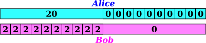
Specifically: Consider the two experimental procedures outlined in figure 3. Alice observes using a 10 minute windown and records a total of 20 events from 1:00 to 1:10, then starts using a 1 minute window and records 0 events in each of the minutes from 1:10 to 1:20. Meanwhile Bob starts out with a 1 minute window, and records 2 events per minute from 1:00 to 1:10, then switches to a ten minute window and observes 0 events from 1:10 to 1:20.
The question is, what’s the best way of doing things? It turns out it doesn’t matter! Here’s why:
Since each reading is statistically independent of the others, the overall probability is just the product of the individual probabilities:
| (12) |
where i runs over all observations.
Our goal (for the moment) is to find the r that maximizes the likelihood. So we will soon take the derivative of P with respect to r, and set it to zero. However, even before we do that, we can simplify things quite a bit:
| (13) |
where the quantity in brackets does not depend on r, and gets thrown away as soon as we set the derivative to zero. The magnitude of the likelihood depends on the bracketed factor, but the value of the optimal r does not.
The upshot is remarkable: The only thing the fitting procedure cares about is the total number of events (Σ ki) and the total time of observation (Σ wi).
This is reminiscent of Raikov’s theorem, although I’m not sure it’s exactly the same.
You can use this for testing your curve-fitting procedures. Make up some data like the Alice and Bob example and feed it to your routine. If it does not cough up r=1 as the maximum-likelihood fit, your routine is broken.
Suppose you have a source that from moment to moment exhibits Poisson statistics, but over time the rate changes. In this situation you really don’t want to have a long observation window. That is, you don’t want the rate to change appreciably during the observation.
The invariance described in this section means you have nothing to lose by using short observation windows. The reading in any particular window will exhibit ugly fluctuations, but the fitting routine doesn’t care. The maximum likelihood calculation will sort everything out.
Forsooth, the whole idea of counting the number of events in an interval is old-fashioned and usually suboptimal. Modern good practice is simply to timestamp the arrival of each and every event.1 In some sense this corresponds to a huge number of windows, each of infinitesimal size ... but it’s simpler to just think of it as timestamping the events.
This is not a solution to the general problem, but only an example ... sort of a warm-up exercise.
Suppose we have a molecule that can be in one of three states, called Bright, Fringe, and Dark. The probability of finding the molecule in each of these states is b, f, and d respectively. Similarly, in each of these states, the variable µ takes on the values B, F, and D respectively. That is,
| (14) |
where those are the prior probabilities, i.e. the probabilities we assign before we have looked at the data. Looking at it another way, these prior probabilities tell us where the molecule is “on average”, and we will use the data to tell us where the molecule is at a particular time.
So now let’s look at the data, and see what it can tell us.
Using the Bayes inversion formula (equation 2), we can write
| P(µ:B | ν:y) = |
| for all y (15) |
Next, we plug equation 3 into the RHS to obtain:
| (16) |
where this is the posterior probability, i.e. the probability we infer after having seen that ν takes on the value y. (If there were more than three states, you could easily generalize this expression by adding more terms in the denominator.)
You can check that this expression is well behaved. A simple exercise is to check the limit where B, F, and D are all equal; we see that the data doesn’t tell us anything. Another nice simple exercise is to consider the case where B is large and the other two rates are small. Then if y is small, we have overwhelming evidence against the Bright state ... and conversely when y is large, the probability of the Bright state closely approaches 100%.
From the keen-grasp-of-the-obvious department: The functional form of P(ν:y | µ:B) (equation 3) is noticeably different from the functional form of P(µ:B | ν:y) (equation 16). The latter is what you want to optimize by adjusting the fitting parameters, given the data.
If there are multiple independent observations, the overall posterior probability will have multiple factors of the form given in equation 16.
If we want something that can be summed over all observations and minimized, take the negative of the logarithm of equation 16.
| (17) |
If (big if!) the data is normally distributed then you can compute the negative-log-likelihood by simply summing the square of the residuals. This is the central idea behind the widely used (wildly abused) “least squares” method. Least squares is unsuitable for our purposes for at least two primary reasons: First of all we want MAP, not maximum-likelihood, and secondly our data is nowhere near normally distributed.
We want least log improbability, not least squares.