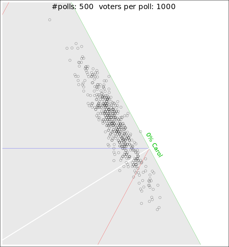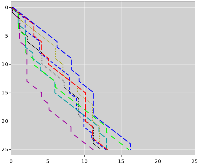
Figure 1: Scatter Plot: Candidates A, B and C
We are often told that a poll of 1000 voters has a “margin of error” on the order of 4%. This is mostly nonsense. The statistical uncertainty (i.e. standard deviation) is at most 1.6% for any particular candidate, and is even less (about 0.3%) for candidates who are polling near 1% (or 99%). Even if you get the math right, it’s still nonsense, since non-statistical uncertainties dominate.
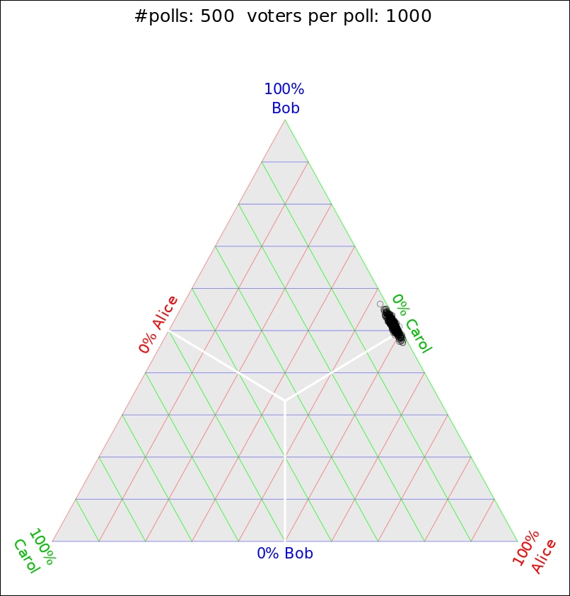
Suppose there are three candidates: Alice, Bob, and Carol. Suppose there are a huge number of voters – more than 100 million – and suppose (somewhat unrealistically) that they have firmly made up their minds. The percentage of the population that favors each candidate is then determined, essentially perfectly, but we won’t know the perfect answer until election day. Until then, we have to make do with polls based on a small sample, perhaps something like 1000 voters.
In particular, suppose the probabilities in the full population are exactly Alice: 47.8%, Bob:51.2%, and Carol: 1%.
We now send pollsters to sample this population. Each sample consists of asking N=1000 voters, randomly selected. Since this is a rather small sample, there will be substantial “sampling error”.
We have three observable variables, namely the sampled A, sampled B, and sampled C. However, they span a space with only two dimensions, because there is a constraint: No matter what, A+B+C has to add up to 100%.
There are powerful techniques for visualizing three variables in two dimensions. A good place to start is a ternary plot, as explained in reference 1.
I did a Monte Carlo simulation of the ABC scenario. Figure 1 shows a scatter plot of the results.
We can learn a tremendous amount from this plot.
A close-up view of the situation is shown in figure 2.
As expected, the data points are most densely clustered in the vicinity of [A, B, C] = [.478, .512, .01].
The meaning of the “standard deviation” (σ) can be understood as follows:
| Interval | Confidence | Roughly | |
| ± σ | 68% | 2 out of 3 | |
| ± 2σ | 95% | 19 out of 20 | |
| ± 2.576σ | 99% | 99 out of 100 |
Here’s an issue that is often underappreciated: In our example, Bob is ahead of Alice by 3.4 points, which you might think is outside the two-sigma error bars, if you think “the” standard deviation for Bob or Alice is 1.6 points. However, the standard deviation of the margin is twice that! That’s because the scores are heavily correlated. Specifically, they are anticorrelated. Alice gains mostly at the expense of Bob, and vice versa. (Alice and Bob can take from Carol a little bit, but not much.) You can see what’s going on by glancing at the figures. A cloud points that is elongated (not round) means there are correlations.
To say the same thing another way, if we think in terms of the standard deviation of Bob’s raw score, he is more than 2σ ahead of Alice – but (!) he is barely 1σ above the tie-line aka the plurality line.
In symbols, we can say, roughly speaking:
| (1) |
In our example, this means that Bob has more than six times as many ways of losing the election than you might have guessed just based on “the” margin and “the” margin of error that the pollsters put out. In figure 2, from Bob’s point of view, there are quite a few dots on the wrong side of the white tie-line.
The main lesson of figure 1 and figure 2 is that there is no such thing as “the” standard deviation for the poll, because different candidates have different standard deviations – and the margins have different standard devations from the raw candidate scores. People have a tendency to get this wrong, whereupon they misunderstand the meaning of the poll.
Constructive suggestion: It’s always better to take a bigger sample, if you can afford it. If you can’t, then you have to closely analyze the data you’ve got.
Specifically, it helps to do use the Monte Carlo method to simulate the situation, as we have done here. One poll produces just one dot in the scatter plot in figure 1 or figure 2. In contrast, Monte Carlo produces lots of dots at a very low cost. That’s a great help in figuring out what the statistics means. Even if you know all the standard deviations, it’s hard for most people to visualize the effect of correlations in a multi-dimensional space.
Not-very-constructive warning: If you think in terms of “error bars on A” and “error bars on B” you are guaranteed to get the wrong answer ... and you won’t even know how grossly wrong it is.
Marginally-constructive suggestion: Look at the covariance matrix, as discussed in section 7.
Recently, on the NPR web site, I saw an article that said in part:
We’ve put together a chart showing how the candidates stack up against each other [...] and how much their margins of error overlap. [...] there’s a +/- 3.8-percentage-point margin of error, so we created bars around each estimate showing that margin of error.
The article (reference 2) supported this point using the graphic in figure 3.
The “error bars” in that diagram are wildly incorrect. This should be obvious from the fact that you can’t possibly have a probability of 1% plus-or-minus 3.8% – for the simple reason that probabilities cannot be negative. The NPR article arbitrarily chops off the part of the error bar that extends below zero, but that is just a way of hiding the problems with the formula they are using.
Let’s be clear: The formula the are using does not apply to this situation. This is an example of what is sometimes called equation hunting in its worst form. That is, somebody hunts up an equation that seems to involve most of the relevant variables, and applies it without understanding it, without realizing that it’s the wrong equation.
By way of background, let’s consider a different situation. Forget about the 679 voters, and instead randomly toss 679 fair coins. Then the average number of heads would be 50% and we can think about the uncertainties as follows:
| Interval | Confidence | Aka | |
| σ = 1.93% | 68% | 2 out of 3 | |
| 2σ = 3.87% | 95% | 19 out of 20 | |
| Σ = 2.576σ = 5.15% | 99% | 99 out of 100 |
So evidently NPR is approximating voters as coins, and using two-sigma error bars. Beware that other pollsters commonly use larger error bars, corresponding to 99% rather than 95% confidence. And scientists almost always quote the standard deviation, σ, from which you can figure out the rest.
The NPR article links to a document (reference 3) that contains somewhat-better formulas, but even it gets the wrong answer, saying “those margins might be a little smaller at the low end of the spectrum” when in fact the margins are definitely smaller by quite a bit.
Also it seems kinda amateurish to round 3.87 to 3.8.
However, we have much bigger problems to worry about.
For starters, voters are not coins. They change their minds – sometimes for good reasons and sometimes otherwise – which means there is no abstract unchanging population from which samples can be drawn. If you repeat the poll a few days later, you are looking at a different population.
Also, voters flat-out lie to pollsters (whereas coins don’t).
Here’s another way in which voters are unlike coins: The probability of heads is very nearly 50%, which means you can calculate the standard deviation as σ = ½√N. However, during a primary, which is the situation that NPR considered, it is common to have a whole gaggle of candidates scoring far, far below 50%. In that case it would be better to calculate σ = √(p(1−p)N). That’s applies to the contest of any one candidate against the rest of the field collectively, and does not account for correlations.
For a finite-sized sample, there will always be sample-to-sample fluctuations ... the so-called sampling error. However, very commonly this is not the only source of uncertainty. There can be methodological mistakes, or other systematic errors.
For the sample presented in figure 3, it is conceivable that the total uncertainty could be on the order of 3.8% ... or it could be much smaller than that, or much larger than that.
In fact, there are eleventeen reasons to think that the data is horribly unreliable. When the none-of-the-above response has a higher frequency than the top two candidates combined, there is good reason to think that the respondents have not made up their minds. This source of uncertainty will not go away, no matter how large you make the sample-size N. If you pose a question to people who don’t know and don’t care, it doesn’t matter how many people you ask.
In any case, there is not the slightest reason to think that the systematic error will be proportional to the statistical uncertainty. It is just ridiculous to use a formula such as 1/√N. If it refers to the statistical uncertainty, it has no meaning, because it’s the wrong formula. If it refers to the total uncertainty, it has even less meaning.
Pollsters are notorious for saying that their results have a «sampling error» equal to 1/√N, where N is the number of respondents surveyed. For example, reference 2 and figure 3 use value 1/√679 = 3.8%.
It must be emphasized that 1/√N is not a real mathematical result. To obtain such a formula, you would have to make four or five conceptual errors. If you arrange these errors just right and sprinkle fairy dust on them, you might kinda sorta obtain a numerically-correct answer under some conditions ... but never under the conditions that apply to figure 3 or figure 4.
Note that the previous two assumptions are not equivalent; indeed they are logically independent. The distribution {1/2, 1/2} satisfies both assumptions; the distribution {1/3, 1/3, 1/3} satisfies the first assumption but not the second; the distribution {1/2, 1/4, 1/4} might satisfy the second but not the first, and the distribution {0.7, 0.2, 0.1} satisfies neither.
It is rather common for pollsters to take an interest in situations where there are two major candidates, both of whom receive approximately 50% support. In such a situation, assumption #2 and assumption #3 are valid, and do not count as mistake. Assumption #4 is a mistake, and introduces an erroneous factor of √2. Assumption #5 is another mistake, and introduces another factor of √2 in the same direction, if we imagine that the score for one candidate goes up while the score for the other candidate goes down. Item #6 miraculously cancels the two previous mistakes, possibly leading to a numerically-correct answer ... but only in this special case.
This result is conceptually unsound. In particular, the 1/√N is bogus, and obviously so. Just as obviously, it is a mistake to treat the two scores as statistically independent. You could equally well apply the same formula to a scenario where both candidates’ scores increase, which has zero probability. It is mathematically impossible. The only real possibility is that one candidate increases at the expense of the other. Any formula that assigns the same probability to the real scenario and the impossible scenario is obviously bogus.
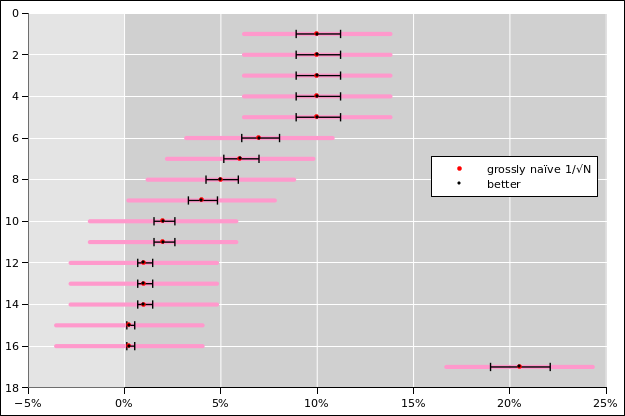
In the multi-candidate scenario presented in figure 3, assumptions #1, #2, and #3 are disastrously wrong. A modestly better formula for the error bar in such a scenario is √(N pi (1−pi)). This result is derived in section 5.2. It reduces to the aformentioned special case 0.5/√N when pi is near 50%, but when pi is small the correction is quite substantial, as you can see by looking at the black error bars in figure 4.
The electoral college system greatly magnifies uncertainty. Small changes in a few key states can have a huge effect on the bottom-line outcome.
The electoral college has plenty of problems, but it’s not as unreasonable as some people make it out to be. The idea of “one person one vote” sounds fine on paper, but in practice it would be bad news for minorities; it would mean they lose the vote every time. There’s no point in having a vote if it doesn’t mean anything. The electoral college was intended to give more voting power to certain minorities. You can’t just abolish it; you have to carefully craft a replacement. The simple solutions are not good, and the good solutions are not simple.
This discussion uses basic probability ideas, as discussed in reference 4.
The whole concept of “error bars” is problematic whenever we are dealing with more than one variable, especially when we know the variables are correlated, extra-especially when the underlying distribution is non-Gaussian. However, let’s temporarily pretend we didn’t notice that, and try to make some modest improvements within the error-bar framework.
The black error bars in figure 4 show a somewhat more reasonable analysis of the situation. There is some overlap of the error bars involving 10th place and 11th place, but there’s nothing special about that; there have been close contests throughout history, for as long as there have been contests. However, my point is, in this case the error bars do not overlap between 9th place and 11th place. Also the error bars do not overlap between 10th place and 12th place. Perhaps more significantly, the error bars for 8th place do not come anywhere near overlapping the error bars for 5th place.
The 17th row in figure 4 shows the ever-popular “none of the above” option. It is worth paying some attention to this, if we want our probabilities add up to 100%.
The error bars are not symmetrical, because they take into account the fact that we don’t know the underlying probability in the global population, and must estimate it from the data. Figure 4 uses the formulas calculated in section 5.4.
Disclaimer: This is not a 100% industrial-strength professional analysis. In particular, it does not take into account correlations. Also it does not properly take into account the prior (aka base rate) on the model parameters. Also it does not account for systematic error (as discussed in section 3.2.) On the other hand, it does use error bars that are in the right ballpark, and it shows how lopsided error bars can arise when estimating model properties from the data.
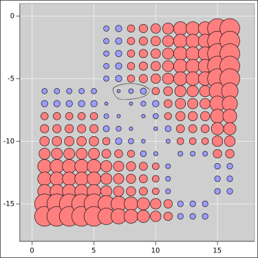
Figure 5 shows how expensive it would be to make a pairwise switch in the rankings, starting from the data in figure 3. Specifically, for each pair of candidates, we start by finding how far apart they are in the standings. We then imagine erasing that split, by moving one of them up by half the split, while moving the other down the same amount.
We leave all other candidates unchanged, because that is the cheapest way to erase the difference.
This maneuver moves us to a less-likely place on the cumulative probability distribution. We express this as a distance, namely the Mahalanobis distance, as defined in equation 36. In other words, we are measuring how far the two candidates are apart, measured in units of the standard deviation, i.e. measured relative to the width of the distribution. We use the full covariance matrix to measure the width in the relevant direction, in the relevant subspace, i.e. the subspace that involves taking from one and giving to the other directly.
In the figure, the area of each bubble is proportional to the Mahalanobis distance. Red coloration indicates that the distance is greater than 3 units. In accordance with the usual formula for the Gaussian cumulative probability distribution, three units covers 99.87% of the normal distribution.
This permits a nice solution to the original political problem. Suppose you think it makes sense a priori to have the six leading candidates on stage ... based on their true standings in the overall population. You cannot directly observe the true standings, so you have to rely on the poll results instead. If you include only the six top-polling candidates, there is some chance that you will exclude one of the guys who should be included. You can see this by reading across the sixth row of the table (or, equivalently, reading down the sixth column). After you accept the top six candidates, there are three more within a not-too-large Mahalanobis distance from the sixth-place guy. That’s a problem, but it can easily be fixed by including those three extra guys, namely the ones that are circled in the figure. Consider them a buffer. There is a very high probability that the six top-true candidates are among the nine top-polling candidates.
Let’s be clear: You can’t pick six guys and be sure they are the true top six. You can however pick nine guys and be very very confident that they include the true top six. Similarly you can pick ten guys and be very confident that they include the true top eight, and super-confident that they include the true top seven. Putting more people on the debate stage would benefit the low-ranking candidates at the expense of the high-ranking candidates. It is reasonable – indeed necessary – to require people to earn a place on the stage. There are plenty of ways of setting a threshold in such a way that one can say with high confidence that anyone below the threshold did not earn a place.
The data in figure 5 is shown in numerical form in table 1.
| -0 | 0 | 0 | 0 | 0 | 1.9 | 2.7 | 3.6 | 4.6 | 6 | 8.1 | 12 | 12 | 12 | 26 | 26 | 4.8 | |||||||||||||||||||
| 0 | -0 | 0 | 0 | 0 | 1.9 | 2.7 | 3.6 | 4.6 | 6 | 8.1 | 12 | 12 | 12 | 26 | 26 | 4.8 | |||||||||||||||||||
| 0 | 0 | -0 | 0 | 0 | 1.9 | 2.7 | 3.6 | 4.6 | 6 | 8.1 | 12 | 12 | 12 | 26 | 26 | 4.8 | |||||||||||||||||||
| 0 | 0 | 0 | -0 | 0 | 1.9 | 2.7 | 3.6 | 4.6 | 6 | 8.1 | 12 | 12 | 12 | 26 | 26 | 4.8 | |||||||||||||||||||
| 0 | 0 | 0 | 0 | -0 | 1.9 | 2.7 | 3.6 | 4.6 | 6 | 8.1 | 12 | 12 | 12 | 26 | 26 | 4.8 | |||||||||||||||||||
| 1.9 | 1.9 | 1.9 | 1.9 | 1.9 | -0 | 0.72 | 1.5 | 2.4 | 3.6 | 5.2 | 8.4 | 8.4 | 8.4 | 18 | 18 | 7.2 | |||||||||||||||||||
| 2.7 | 2.7 | 2.7 | 2.7 | 2.7 | 0.72 | -0 | 0.79 | 1.7 | 2.8 | 4.3 | 7 | 7 | 7 | 15 | 15 | 8.2 | |||||||||||||||||||
| 3.6 | 3.6 | 3.6 | 3.6 | 3.6 | 1.5 | 0.79 | -0 | 0.87 | 1.9 | 3.3 | 5.7 | 5.7 | 5.7 | 13 | 13 | 9.5 | |||||||||||||||||||
| 4.6 | 4.6 | 4.6 | 4.6 | 4.6 | 2.4 | 1.7 | 0.87 | -0 | 1 | 2.3 | 4.4 | 4.4 | 4.4 | 10 | 10 | 11 | |||||||||||||||||||
| 6 | 6 | 6 | 6 | 6 | 3.6 | 2.8 | 1.9 | 1 | -0 | 1.2 | 3 | 3 | 3 | 7.5 | 7.5 | 13 | |||||||||||||||||||
| 8.1 | 8.1 | 8.1 | 8.1 | 8.1 | 5.2 | 4.3 | 3.3 | 2.3 | 1.2 | -0 | 1.6 | 1.6 | 1.6 | 4.8 | 4.8 | 17 | |||||||||||||||||||
| 12 | 12 | 12 | 12 | 12 | 8.4 | 7 | 5.7 | 4.4 | 3 | 1.6 | -0 | 0 | 0 | 2.2 | 2.2 | 25 | |||||||||||||||||||
| 12 | 12 | 12 | 12 | 12 | 8.4 | 7 | 5.7 | 4.4 | 3 | 1.6 | 0 | -0 | 0 | 2.2 | 2.2 | 25 | |||||||||||||||||||
| 12 | 12 | 12 | 12 | 12 | 8.4 | 7 | 5.7 | 4.4 | 3 | 1.6 | 0 | 0 | -0 | 2.2 | 2.2 | 25 | |||||||||||||||||||
| 26 | 26 | 26 | 26 | 26 | 18 | 15 | 13 | 10 | 7.5 | 4.8 | 2.2 | 2.2 | 2.2 | -0 | 0 | 50 | |||||||||||||||||||
| 26 | 26 | 26 | 26 | 26 | 18 | 15 | 13 | 10 | 7.5 | 4.8 | 2.2 | 2.2 | 2.2 | 0 | -0 | 50 | |||||||||||||||||||
| 4.8 | 4.8 | 4.8 | 4.8 | 4.8 | 7.2 | 8.2 | 9.5 | 11 | 13 | 17 | 25 | 25 | 25 | 50 | 50 | -0 |
Disclaimer: This is not a 100% industrial-strength professional analysis. In particular, it does not take into account the fact that the distribution is not Gaussian. Also it does not account for systematic error (as discussed in section 3.2.) On the other hand, it does use error bars that are in the right ballpark, and it shows how correlations can give rise to a distribution that is elongated in some directions, and rotated relative to the “natural” variables.
The goal is to understand the statistics of public-opinion polling. In particular, we want to know how much uncertainty attaches to the results, purely as a result of sampling error. (We ignore the all-too-real possibility of methodological problems and other systematic errors.)
Rather than attacking that problem directly, let’s start by doing a closely-related problem, namely the random walk (section 5.1). Once we have figured that out, the solution to the original problem is an easy corollary (section 5.2).
A random walk is reasonably easy to visualize. The mathematics is not very complicated.
The walk involves motion in D dimensions. At each step, the walker moves a unit distance in one of the D possible directions; there are no diagonal moves. The probability of a step in direction i is pi, for all i from 0 through D−1 inclusive.
The situation is easier to visualize if we imagine some definite not-very-large value if D, but mathematically the value of D isn’t very important. We can always imagine an extra-large value for D, and just set pi=0 for each of the extra dimensions.
This pi represents the underlying probability in the global population. In any particular walk, we do not get to observe pi directly.
Each walk consists of N steps. To keep track of the wallker’s position along the way, we use the vector variable x which has components xi for all i from 0 to D−1. More specifically, we keep track of x(L) as a function of L, where L is the number of steps in the walk, from L=0 to L=N.
To define what we mean by sampling error, we must imagine an ensemble of such walks. There are M elements in the ensemble.
Table 2 shows the position data x(L) for eight random walks. This shows what happens for only one of the dimensions; the table is silent as to what is happening in the other D−1 dimensions.
| walk | #1 | #2 | #3 | #4 | #5 | #6 | #7 | #8 | |
| length | |||||||||
| 0 | 0 | 0 | 0 | 0 | 0 | 0 | 0 | 0 | |
| 1 | 0 | 0 | 0 | 0 | 0 | 0 | 1 | 1 | |
| 2 | 0 | 1 | 1 | 0 | 0 | 0 | 2 | 1 | |
| 3 | 1 | 2 | 1 | 1 | 0 | 0 | 3 | 1 | |
| 4 | 1 | 2 | 2 | 2 | 1 | 1 | 4 | 2 | |
| 5 | 1 | 3 | 3 | 2 | 1 | 1 | 4 | 2 | |
| 6 | 2 | 3 | 4 | 3 | 2 | 1 | 5 | 3 | |
| 7 | 2 | 3 | 4 | 4 | 2 | 1 | 6 | 3 | |
| 8 | 2 | 4 | 4 | 5 | 2 | 2 | 6 | 3 | |
| 9 | 2 | 4 | 4 | 6 | 2 | 2 | 7 | 4 | |
| 10 | 3 | 4 | 5 | 7 | 2 | 3 | 7 | 4 | |
| 11 | 4 | 5 | 6 | 8 | 3 | 4 | 8 | 5 | |
| 12 | 4 | 5 | 6 | 9 | 4 | 4 | 8 | 6 | |
| 13 | 4 | 5 | 7 | 9 | 5 | 5 | 9 | 7 | |
| 14 | 5 | 6 | 8 | 9 | 6 | 5 | 10 | 7 | |
| 15 | 5 | 6 | 9 | 9 | 6 | 5 | 10 | 7 | |
| 16 | 5 | 6 | 9 | 9 | 6 | 6 | 10 | 7 | |
| 17 | 6 | 7 | 9 | 9 | 6 | 7 | 10 | 7 | |
| 18 | 6 | 8 | 10 | 10 | 7 | 7 | 10 | 7 | |
| 19 | 7 | 8 | 11 | 10 | 7 | 8 | 11 | 8 | |
| 20 | 7 | 8 | 11 | 10 | 7 | 9 | 12 | 9 | |
| 21 | 7 | 8 | 11 | 10 | 7 | 9 | 12 | 10 | |
| 22 | 7 | 9 | 11 | 11 | 7 | 9 | 13 | 11 | |
| 23 | 8 | 9 | 11 | 12 | 7 | 10 | 14 | 12 | |
| 24 | 9 | 9 | 11 | 13 | 7 | 10 | 14 | 13 | |
| 25 | 10 | 9 | 11 | 13 | 7 | 11 | 14 | 13 |
Figure 6 is a plot of the same eight random walks.
We now focus attention on the x-values on the bottom row of table 2. When we need to be specific, we will call these the x(N)-values, where in this case N=25. It turns out to be remarkably easy to calculate certain statistical properties of the distribution from which these x-values are drawn.
The mean of the x(N) values would be nonzero, if we just averaged over the eight random walks in table 2. On the other hand, it should be obvious by symmetry that the mean of the x(N)-values is zero, if we average over the infinitely-large ensemble of possible random walks with the given population-base probabilities pi.
We denote the average over the large ensemble as ⟨⋯⟩. It must be emphasized that each column in in table 2 is one element of the ensemble. The ensemble average is an average over these columns, and many more columns besides. It is emphatically not an average over rows.
Consider the Lth step in the random walk, i.e. the step that takes us x(L−1) to x(L). Denote this step by Δx. For each i, there is a probability pi that xi is +1 and a probability (1−pi) that it xi is 0.
The calculation goes like this:
To obtain the last line, we used the fact that xi(0) is zero, and used induction on L. We see that on average, each step of the walk moves a distance pi the ith direction.
To understand the spread in the distribution, let’s look at some second-order statistics. We define a new variable
| (3) |
that measures how far our random walker is away from the ensemble-average location.
| (4) |
To derive the last line, we used the fact that ⟨(Δxi − pi)⟩ is zero ... and is independent of y(L−1).
Let’s start by considering the case where i=j. Then the result of equation 4 simplifies to
|
To get to equation 5b we used the fact that Δxi is 1 with probability pi, and is 0 with probability (1−pi). To get to equation 5d, we used the fact that yi(0)2 is zero, and used induction on L. This gives us the mean-square distance of the ith coordinate from its average value. (The “mean” in this mean-square distance is the ensemble average.)
Equation 5d is related to a famous result. If we divide by L2, it gives us the variance of a generalized Bernoulli process. Note that a simple Bernoulli process is a model of a coin toss, with two possible outcomes (not necessarily equiprobable). A generalized Bernoulli process a model of a multi-sided die, with D possible outcomes (not necessarily equiprobable).
A generalized Bernoulli distribution is sometimes called a categorical distribution or a multinomial distribution.
For the off-diagonal case, i.e. i≠j, there are three possibilities:
We can say the same thing in mathematical terms, as follows:
|
To obtain equation 6d, we once again used induction on L.
It is conventional and reasonable to report the results of a poll in terms of the average over all responses. This differs from a random walk, which we formulated in terms of a total tally (rather than an average).
To obtain the relevant average, all we need to do is set L=N in equation 2c and then divide both sides by N. That is, we define the vector
| (7) |
and therefore in accordance with equation 2c
| (8) |
To measure the spread relative to the mean, we apply a similar factor of 1/N to equation 3, which gives us:
| (9) |
The variance (i.e. the diagonal part of the covariance) is
| (10) |
and the rest of the covariance is
| (11) |
When the probability is near 50%, equation 10 yields a familiar formula for the standard deviation:
| (12) |
This can be compared with equation 33.
Consider the case where there are only two dimensions, i.e. D=2. This corresponds to an ordinary coin toss. Now suppose the coin is bent, so that at each step the two possible outcomes are unevenly distributed, with a 60:40 ratio. Then the covariance matrix is exactly:
| (13) |
This Σ is called the covariance matrix. The elements on the diagonal are called the variances. The square root of the variance is called the standard deviation. You can see that the standard deviation is σi = √(pi(1−pi)/N). The usual moderately-naïve practice is to set the so-called error bars equal to the standard deviations determined in this way. This is better than assuming 0.5/√N and vastly better than assuming 1.0/√N ... but still not ideal, because the whole idea of “error bars” is flawed.
In two dimensions, the numbers are particularly simple because in two dimension, there are only two probabilities, and pj = (1−pi). Therefore the diagonal elements pi (1−pi) and the off-diagonal elements −pi pj have all the same magnitude.
This is one of those rare cases where you can do the SVD in your head. The normalized eigenvectors and the corresponding eigenvalues are
| (14) |
You can see that for a fluctuation in the “cheap” direction, the error bar is longer by a factor of √2 compared to what you would expect by naïvely ignoring correlations. In the “expensive” direction, the error bar is shorter by a factor of infinity.
Consider a public opinion poll where there are three candidates. A and B each have 49% support, while C has the remaining 2%. This is the scenario depicted in figure 1. The covariance matrix is:
| (15) |
The unit eivenvectors are:
| (16) |
And the corresponding eivenvalues are
| (17) |
So the oriented error bars are:
| (18) |
The first errror bar corresponds to a purely horizontal motion in figure 1, while the second corresponds to a purely vertical motion.
Suppose we survey N respondents, and none of them report being in favor of candidate A. We assume A actually has some nonzero favorability p in the global population, and we missed it due to sampling error. Let’s calculate the probability of that happening.
When a respondent does not favor A, we call it a miss. The chance of the first responding missing A is (1−p). There is some chance of getting N misses in a row, which we denote θ. We can calculate:
| (19) |
As a numerical example, suppose that A has a true population-based probability p equal to half a percent, and suppose the sample-size is N=600. Then in 5% of the samples, there will be zero observations of A. For larger sample sizes, the probability of completely missing A goes exponentially to zero, but when p is small, N has to get quite large before the exponential really makes itself felt.
By turning the algebraic crank, we can solve equation 19 for N. That gives us:
| (20) |
assuming p is small compared to unity. Equation 20 is a moderately well-known result. Turning around the previous numerical example, if you want to run at most a 5% risk of missing A, then the numerator on the RHS of equation 20 is 3. (Remember that e cubed is 20, to a good approximation.) Therefore if the true population-based probability is half a percent, the sample size had better be at least 600.
Turning the crank in the other direction, one could perhaps obtain:
| (21) |
Alas this equation is open to misinterpretation, to say the least. The p in equation 21 probably doesn’t mean the same thing as the p in equation 20. In particular, it would be more-or-less conventional to interpret equation 19 as some sort of conditional probability of getting N misses, conditioned on θ and p:
| (22) |
In contrast, it would be more-or-less conventional to interpret equation 21 as some sort of conditional probability of p, conditioned on θ and N:
| (23) |
See section 6 for further discussion of the notational and conceptual problems with equation 21.
Before we can find a reasonable equation for p, we need to understand the prior distribution of p-values, and take that into account, presumably by use of the Bayes inversion formula (equation 26).
Here is an example of the sort of max-a-posteriori question we would like to ask: Given some small threshold θ, we would like to find some є that will allow us say with high confidence (1−θ) that the true probability p is less than є.
It is possible to answer such a question, but it’s more work than I feel like doing at the moment.
Results such as equation 10 and equation 11 apply in the rather unlikely scenario where some oracle has told us the true value of the probability p in the general population. More generally, we can consider p to be the parameters of the model, and we are calculating the a priori probability:
| (24) |
Note that this particular a priori probability is technically called the likelihood. Note that “likelihood” is definitely not an all-purpose synonym for probability. This is a trap for the unwary.
In the usual practical situations, we don’t know p, and we are trying to estimate it from the data. This corresponds to calculating the a posteriori probability:
| (25) |
One way to calculate such this is via the Bayes inversion formula:
| (26) |
The marginal P[data]() in the denominator on the RHS is the least of our worries. It serves as a normalization factor for the RHS as a whole. If it were the only thing we didn’t know, we could calculate it instantly, just by doing the normalization.
In contrast, the marginal P[model]() in the numerator on the RHS is very often not known, and not easy to calculate. In general, this is an utterly nontrivial problem. Sometimes it is possible to hypothesis a noncommittal “flat prior” on the parameters of the model, but sometimes not.
As a first step in the right direction, let’s take another look at equation 8 and equation 10. Rather than thinking of the observed data as a±b in terms of a known p, let us ask what values of p are consistent with the observed a.
We can use a itself as an estimator for the middle-of-the-road nominal value of p, by inverting equation 8.
| (27) |
Note the subtle distinction; if we knew p a priori we would use equation 8 to calculate a. In contrast, here we start with an observed value for a, and then use equation 27 to estimate the nominal value of p.
Using the same logic, if we knew p a priori we might use equation 10 to calculate an error bar, disregarding correlations. In contrast, here we start with an observed value for a, and obtain an estimate for the top of the high-side error bar on a by solving the following equation:
| (28) |
where the length of the error bar is given by the second term on the RHS, i.e. the square-root term. The whole idea of «error bars» is conceptually flawed, but let’s ignore that problem for the moment. In equation 28, we are seeking the high-side error bar on a, which corresponds to the low-side error bar on phigh. Conceptually, we are searching through all possible phigh values to find one whose low-side error bar extends down far enough to reach a. The length of the error bar is calculated from equation 10 by plugging in the value of phigh ... emphatically not by plugging in the value of pnom.
Similarly the low-side estimate of p is found by searching through all possible values for plow to find one whose high-side error bar extends up far enough to reach a.
| (29) |
Let’s turn the crank on the algebra:
| (30) |
We finish the solution using the quadratic formula:
| (31) |
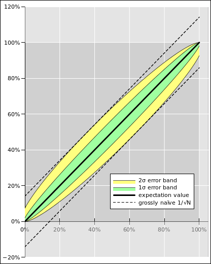
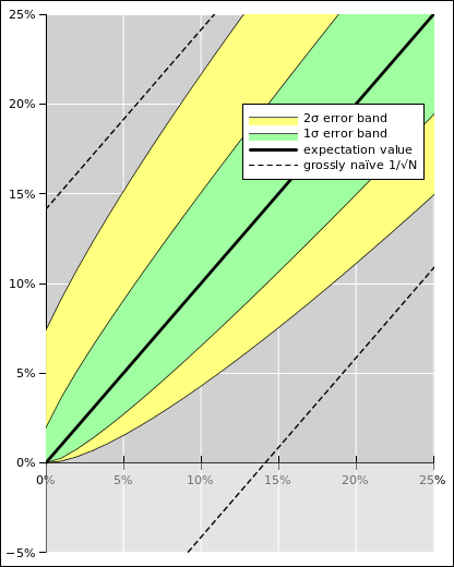
If you want to increase the confidence level, you can find the kσ error bar (instead of the conventional 1σ error bar) by replacing N by N/k2 in all of these formulas.
The results are plotted in figure 7 and figure 8. The figures show the conventional 1σ error band in green, and show the 2σ error band in yellow. Also, for comparison, the dotted lines in the figures figures show the grossly naïve error bars used in the NPR article, namely the 3.8% error bars based on the 1/√N formula.
Some observations:
In the special case where a is very small, equation 30 simplifies to
| (32) |
which is of the same form as equation 21, where the confidence level is θ=exp(−k2).
Note that when p is known, the uncertainty on a is zero when p=0, in accordance with equation 10 ... whereas when a is known, the uncertainty on p is definitely not zero, even when a is zero, in accordance with equation 32, assuming N is finite. This is an important and utterly nontrivial conceptual point.
For a=0, this reduces to equation 32. For a=0.5, it reduces to
| (33) |
which gives the same result as equation 12 in the large-N limit ... whereas for small N it is different.
When a=1, this reduces to
| (34) |
which makes sense. The top of the error bar cannot ever be greater than p=1 ... and also it cannot be less than a, so for a=1 the error bar is quite well pinned down.
The calculations for plow are very similar, except we are interested in the other root of the quadratic. The results exhibit a mirror-image symmetry. You can easily verify that for a=0, the lower error bar is zero; for a=0.5 the lower error bar has length 0.5/√N, and for a=1 the lower error bar has length 1/N.
The formulas we have just calculated correspond to the Wilson interval (as discussed in e.g. reference 3). This is certainly not the most sophisticated way of defining the confidence interval ... but it is better than the 3.8% error bars that were blindly assumed in figure 3, better by at least two large steps in the right direction.
Note that the naïve notion that the length of the error bar “should” be inversely proportional to √N only works when the probability is near 50% ... and fails miserably otherwise, as we see in figure 4.
Professional statisticians spend enormous amounts of time just staring at data. They cover the walls of their office with plots. If the first representation doesn’t tell the tale, they construct another, and another, and another.
As a corollary: If you have three variables with a constraint, a ternary plot such as figure 1 might be just the ticket. It takes a few hours of staring at such things before you get good at interpreting them ... so don’t panic if it’s not 100% clear at first sight. See reference 1.
The code I used for this little project is given in reference 6 and reference 7.
It’s no wonder that people find probability and statistics to be confusing. The ideas aren’t particularly complicated, but the terminology stinks and the notation stinks.
Let’s look aat the covariance matrix. This is one of necessary (but not sufficient) things you must do if you want to talk about uncertainty with any pretense of professionalism. The formula for a multi-dimensional Gaussian can be written
| (35) |
where dP is the probability density distribution, and dM is the Mahalanobis distance, which is defined in terms of the covariance matrix Σ:
| (36) |
The R vector is the independent variable in the problem at hand. For the example discussed in this section and in section 5.2.2, the components of R are the A, B, C variables we used to define the problem. That is:
| (37) |
As always, R⊤ denotes the transpose of R. If R is a column vector, R⊤ is a row vector. As a corollary, this means that A⊤ B is the dot product A·B (for any two vectors A and B). Also, Σ−1 denotes the matrix inverse of Σ ... or if necessary, the pseudoinverse.
Equation 35 is the natural generalization of the familiar expression for a one-dimensional Gaussian:
| (38) |
In simple cases, the covariance matrix will be more-or-less diagonal using whatever variables you have chosen. Then each diagonal element is the variance i.e. σ2 for the corresponding variable. In such a case, congratulations; you can continue using those variables without too much hassle. However, alas, the problems that land on my desk are almost never simple. In the present case, the covariance matrix is mess. There are tremendous off-diagonal elements. These indicate correlations. Indeed, the correlations are so bad that the matrix is singular, and Σ−1 does not even exist, strictly speaking.
I said that looking at the covariance matrix is "marginally" constructive because (by itself) it provides little more than a warning. It’s like a sign that says you are in the middle of a minefield. You know you’ve got a big problem, but can’t solve it without additional skill and effort.
Singular Value Decomposition sometimes offers you a way out of the minefield. It is especially useful if the data is Gaussian distributed ... and it might provide some qualitative hints even in non-Gaussian situations.
SVD is one of those things (rather like a Fourier transform) that you cannot easily do by hand ... but you can compute it, and then verify that it is correct, and then understand a lot of things by looking at it. In particular, given the SVD, it is trivial to invert the matrix; keep the same eigenvalues, and take the arithmetical reciprocal of the eigenvectors.
Specifically, SVD will give you the eigenvectors and the corresponding eigenvalues of the covariance matrix Σ. In our example, the raw covariance matrix is:
| (39) |
If you unwisely ignore the off-diagonal elements and take the diagonal elements (i.e. the variances) to be the squares of the error bars, you get
| (40) |
For two of the variables we (allegedly) have 7% uncertainty. This is half of what pollsters conventionally quote. Beware that 7% is wrong, as discussed below. Meanwhile 14% is conceptually wrong, for a different reason ... unless you are willing to make three mistakes that cancel each other out. As a separate matter, note that the alleged uncertainty on C is only 2%. That’s not as crazy as 14%, but it’s not exactly right, either.
The eigenvectors of Σ are:
| (41) |
and the corresponding eigenvalues are
| (42) |
The third eigenvalue is actually zero. Because of roundoff errors it is represented here by a super-tiny floating-point number. The zero eigenvalue corresponds to a zero-length error bar in a certain direction. It tells that if we change A by itself, keeping B and C constant, we violate the constraint that A+B+C must add up to 1. Ditto for changing B or C by itself. This corresponds to moving in the third dimension in the ternary plot, i.e. leaving the plane of the paper. It is not allowed. In accordance with equation 38, any movement at all in the direction of a zero-length error bar will cause the probability to vanish.
The first eigenvector is the "cheap" one. You know this because it corresponds to the large eigenvalue of Σ (and hence the small eigenvalue of Σ−1). To a good approximation, it represents increasing A at the expense of B (and/or vice versa) along a contour of constant C. You know this by looking at the eigenvector components in the first column. SVD is giving us a lot of useful information.
Taking the square root of the eigenvalue, we find that the error bar is 9.9% in the cheap direction ... not 7% and not 14% but smack in between (geometric average). Meanwhile the calculation suggests an error bar of 2.4% in the other direction, i.e. increasing C and the expense of A and B equally. Alas, this is not as useful as one might have hoped, because the distribution is grossly non-Gaussian in this direction. Starting from the peak of the distribution, can move several times 2.4% toward the north, but we cannot move even one times 2.4% toward the south.
Overall, we can get a fairly decent handle on whats going on using a combination of Monte Carlo, ternary plots, and Singular Value Decomposition.