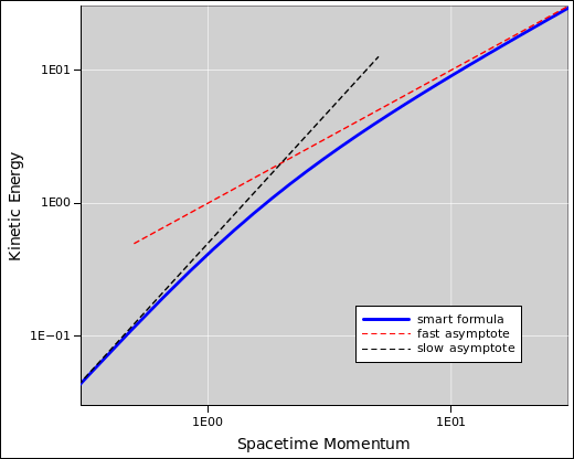
Figure 1: Spacetime Kinetic Energy
Suppose we want to calculate the kinetic energy of a particle, as a function of momentum, over a wide range that includes relativistic speeds as well as non-relativistic “table-top” speeds. Doing this properly requires knowing some basic things about computational physics and numerical methods in general.
As a check, we know that in the non-relativistic limit, we have
| (1) |
and in the relativistic limit we have
| (2) |
with no factor of one-half.
However, we want to know what happens across the whole range, fast, slow, and (!) in between.
The easy part can be expressed in terms of the rapidity, ρ. We use the concepts and the notation from reference 1.
| (3) |
For simplicity we set c=1 and set m=1 from now on. You can easily enough stick the factors of c and m back in, but this is left as a further exercise for the reader.
If we don’t care about well-behaved numerical evaluation, the obvious energy formulas are:
| (4) |
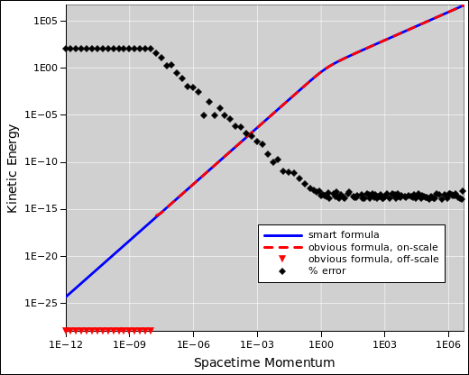
Equation 4 is algebraically correct, but it is not numerically well behaved. If you evaluate it by hand, using “significant figures” ideas, it will give the wrong answer for any smallish ρ. Even if you use a spreadsheet or typical programming language, using IEEE double-precision, equation 4 is worse than useless at table-top speeds, i.e. when ρ is small, on the order of 10−8 radians or less, as we shall see in figure 1.
Subtractions are always bad from a numerical-methods point of view. This is the infamous problem of a “small difference between large numbers”.
You could evade this problem by using two formulas, ½ mv2 for low speeds and something else for high speeds. However, that gets messy in the in-between regime, because at each point you have to ask whether the low-speed approximation is accurate, or the high-speed approximation, or both, or neither. It would be nice to have a single formula that covers the whole range. It’s not a priori obvious that such a formula exists, but it’s certainly worth a try.
Let’s cut to the chase. Consider the following expression, which is algebraically equivalent to the previous expression, but much better behaved numerically:
| (5) |
This formula is trivial to verify a posteriori. Expand the numerator using the Pythagorean trig identity, then divide.
| (6) |
Deriving it ab initio takes a little bit of cleverness, but only a little, once you realize that you want to derive it. The crucial step is realizing that yes, you do want to derive it. The rationale is simple: Putting cosh plus one in the denominator is numerically better behaved than putting cosh minus one in the numerator. Waaaay better. It avoids the problem of “small difference between large numbers”.
Tangential remark: This is related to the distinction between the unsophisticated “textbook” version and the smart version of the quadratic formula, as discussed in reference 2. There exists a quadratic expression that you can solve for the KE.
Figure 1 compares the two approaches. Using IEEE double precision, equation 4 produces wildly wrong answers at table-top speeds, when ρ is small, on the order of 10−8 radians or less. When the wrong answer is zero, it cannot be properly plotted on log-log axes; these data points are approximated by downward-pointing triangles.
This illustrates the point that algebra and numerical evaluation work together. It’s not an either-or situation.
The “corner” in figure 1 is not really a sharp corner. If you zoom in, as in figure 2, you can see there is a gradual change in slope.
For pedagogical reasons makes sense to examine the quadratic formula (reference 2 before diving into this exercise.
Even so, this exercise is not ideal. I am reminded of the proverb that says:
Learning proceeds from the known to the unknown.
That’s a problem, because students who don’t know much relativity will struggle with this example. On the other hand, for students who do know some relativity, this reinforces what they know, and serves as a 100% authentic example of a numerical-methods problem that crops up when doing physics.
So, as usual, we get to apply the proverb that says:
The rich get richer and the poor get poorer.