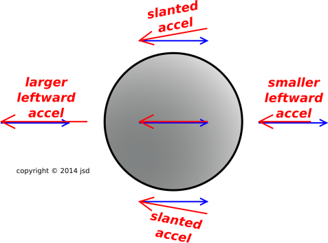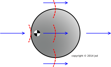
Figure 1: Total Acceleration
The tides are the response of the earth to a driving force that comes from the gravitational field of the moon and sun. For simplicity, let’s consider a day when the sun and moon are aligned, as seen from the earth (i.e. new moon). The sun rises and sets only once per day. So why do most places get two high tides and two low tides on this day (and every other day)? This is discussed in the following sections.
On the other hand, sometimes we do get only one tide cycle per day; the reasons for this are discussed in section 7.
People often miss the following distinction: You need to distinguish
This distinction can be explained in a number of ways. Let’s start with the pictorial approach, as shown in figure 1. The moon is somewhere off to the left. The gravitational acceleration is stronger on the left side of the planet than on the right, because it is inversely proportional to distance squared, in accordance with the law of universal gravitation.
Meanwhile, the acceleration vectors above and below the planet have about the same magnitude as the average acceleration, but the directions are different.
Key idea: A planet subjected to a truly uniform pull would feel no tidal effects whatsoever. If you are standing on a scale and both you and the scale are in free fall, the scale reads zero.
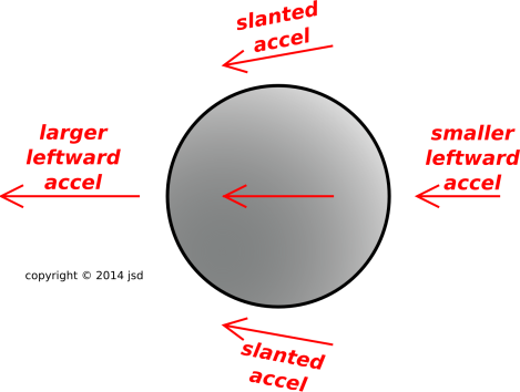
The average pull toward the moon is balanced by the earth’s orbital motion. That’s a solved problem, and is of no further interest when calculating the tides, but if you want the details, see section 6.1. The only thing that matters for the tides is the deviation from the average. So let’s see what happens if we subtract the average from each of the vectors. The negative of the average is shown in blue figure 2.
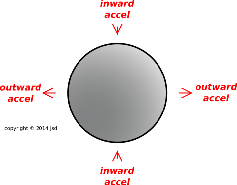
Now let’s perform the subtraction, by adding the local acceleration to the negative of the average, adding the vectors tip-to-tail. That gives us the result shown in figure 3.
We can summarize the diagrams in words, as follows:
This explains why there is a large twice-a-day (semi-diurnal) component to the tide-producing force. Larger-than-average to the right is the same as lower-than-average to the left. Both produce an outward force. It must be emphasized that here we are talking about the tide-producing force; the observed height of the tides is something quite different, as discussed in section 5.1.
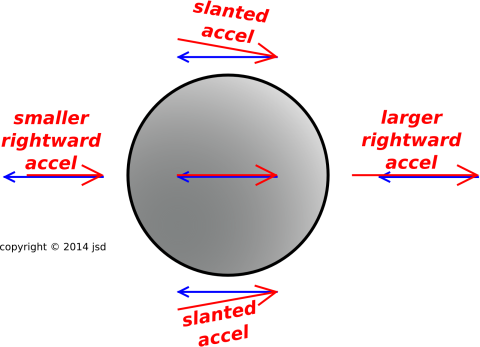
Figure 2 applies when the moon is on the left. Half a month later, the moon will be on the right. This is shown in figure 4. If you do the subtraction, you find that the net tidal acceleration is the same as what we see in figure 3.
Let’s try to understand this using basic principles of physics and a little bit of algebra. (This would be a whole lot easier using calculus, but we can manage without it.)
We start with the famous “elevator” experiment. Suppose you are in an elevator. You set a scale on the floor of the elevator, and place a massive test object on the scale. Now suppose the elevator starts freely falling. The scale will read zero. In the reference frame comoving with the elevator, you are weightless, the scale is weightless, and the test object is weightless.
The same principle applies to planets and everything else. The center-of-mass of the earth is in free fall toward the moon. If we subtract out the earth’s gravity, a test object (or an ocean) at the surface of the earth is also in free fall toward the moon. If the earth and the test object were accelerating at the same rate, there would be no observable consequences, i.e. no tides.
Therefore the only thing that could possibly contribute to the tide-producing stress is the difference between the acceleration of the earth and the acceleration of the test object. This is a direct consequence of the equivalence principle.
To repeat: The tides don’t care about the overall magnitude of the moon’s gravitational field near the earth. The only thing that could possibly matter is the difference between the field at the center and the field at the surface.
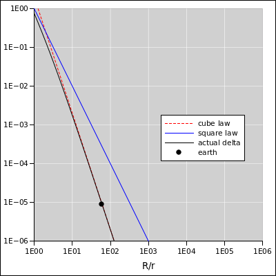
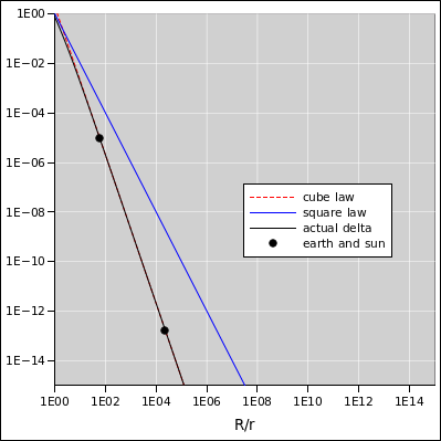
Next we make a scaling argument. The moon is about 60 earth-radii away. The gravitational field scales inversely like distance squared, but we don’t care about that. What we care about is the difference between 1/602 and 1/612. Now it turns out that as a general rule, the difference between 1/(x)2 and 1/(x+1)2 scales like 2/(x)3, when x is not too small.
If you don’t believe me, you can check for yourself. The results should look like figure 5. Also figure 6 shows the same data, only zoomed out to show how it applies to the sun also. The sun is about 23481 earth-radii away. In the figures, the black line represents the actual difference between 1/(x)2 and 1/(x+1)2. The dashed red line is the approximation, namely 2/(x)3, which you can see is a good approximation.
To summarize: Even though the moon’s gravity scales inversely like distance squared, the tidal stress scales inversely like distance cubed.
Globally, the gravitational potential is funnel-shaped. Locally, it is saddle-shaped. The gravitational field is the slope of this potential.
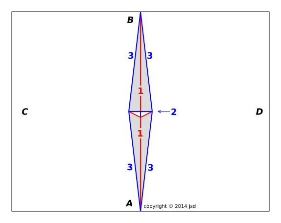
If you have trouble visualizing a saddle-shaped potential, here’s something that may help: Start with a piece of paper. Ordinary 8x11.5 copier paper will do. If you have a supply of fancy origami paper, that’s even better. We want to fold it as shown by the colored lines in figure 7. The blue lines represent peaks, while the red lines represent valleys. Note that the midline of the unshaded triangle is a peak, not a valley.
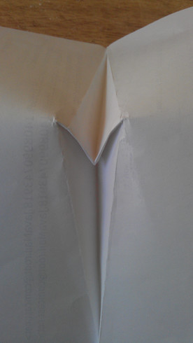
Figure 8 shows the result, slightly unfolded. The sharp edge that we are seeing almost edge-on is fold #2, i.e. the base of unshaded triangle in figure 7. The other sides of the unshaded triangle are tucked up out of sight.
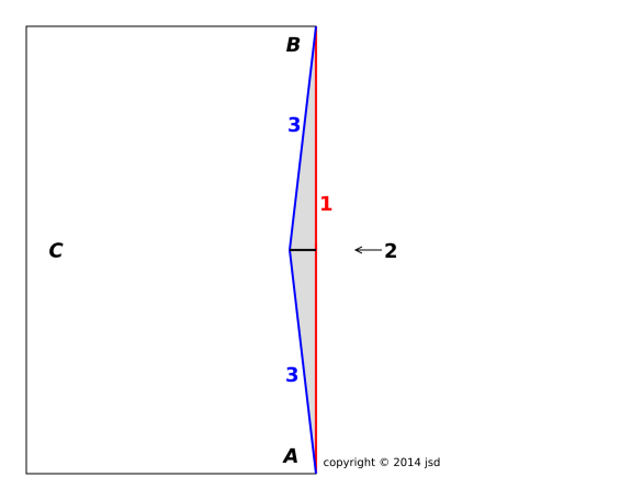
Note: If you are really lazy, you can replace fold #2 by a cut. After making fold #1, while the paper is still folded, make a cut 1/2 inch long as shown by the short black line in figure 9. I consider this considerably less elegant than the origami approach, but it gets the job done.
Hold the model so that you are looking more-or-less along the line from point A to point B (as labeled in figure 7). Observe the curvature of the model.
Imagine five test particles, one at the midpoint and one at each of the labeled points A, B, C, and D. The particles are moving under the influence of the saddle-shaped potential. (They are not big enough to be the source of any appreciable gravitational fields of their own.) Particles C and D will be squashed toward the middle by the concave-upward potential. Meanwhile, particles A and B will be pushed apart by the concave-downward potential.
You can create a model of the funnel-shaped 1/|R| potential, going all the way around the central source, by taping together many of these saddles, joining point C of one saddle to point D of the next.
In the previous section we talked about curvature and gravitation in the same breath, but we are not talking about general relativity. Absolutely not.
The curvature of the potential, as we see here, is wildly different from the curvature of spacetime itself, which is the subject of general relativity. For an introduction to what spacetime curvature looks like, see reference 1.
You know that any function y(x), if it’s not too wild, can be approximated by a polynomial. The same is true in higher dimensions. In this case, we want to represent the potential as a function of two position-variables. (We are forced to omit the third spatial dimension from our model.) The polynomial will have the form
| (1) |
The constant piece is uninteresting. A constant potential no forces.
The planar piece produces a uniform gravitational pull. It holds earth in its orbit around the moon. This is the easy part. You can illustrate this with a flat piece of cardboard. Let a marble roll down the tilted plane, to illustrate the relationship between tilted potential and force.
The saddle-shaped piece produces tides. The math is worked out in section 6.2 and section 6.3.
So far, we have only discussed the field that drives the tides. Now we must ask how the water responds to this driving field. This is a different question entirely.
Imagine a tray containing a thin layer of water. Tilt the tray briefly, then return it to level. The water won’t move very much. But if you tilt it and hold it that way, all the water will move to the low end. So it is with the tides. The lunar and solar gravitational fields effectively tilt the earth’s gravitational potential, changing the local notion of what “horizontal” means.
Let us imagine, temporarily, a planet that is earth-like except that it spins very slowly: slowly compared to the sloshing resonance frequency of all the oceans and bays, and also slowly compared to any viscous relaxation times. On such a planet, the water would come to equilibrium and would map out the potential for us.
However, the slow-spin approximation is a terrible approximation for the real earth. In the equation of motion there are inertia terms, damping terms, and restoring-force terms, none of which are negligible. Each body of water is, to a first approximation, an oscillator. The drive is a complicated function, with components at different frequencies, most of which don’t match the natural frequency of the oscillator.
It is laborious but relatively straightforward to calculate how the water is being driven; It is a much more complicated to figure out how fast and how far the water will move when it is driven. It depends on
It is fairly common for people to think that there should only be one tide cycle per day. The fallacious argument goes something like this: the water is attracted to the moon, so there should be a bulge on the side facing the moon, and a deficit on the opposite side of the earth.
This is fallacious at least two times over. For one thing, it fails to distinguish between the tide-producing potential and the water’s reaction to that potential, as discussed in section 5.1.
But there is a more fundamental fallacy here. Even if we were dealing with a slowly-rotating planet, on which the water could exactly follow the potential, it would be completely fallacious to think that the water bulges up on the moon-facing side and thins out on the opposite side. This is just completely wrong physics.
It is easy to fall into this trap if you think of the earth as being fixed in space, or if you think that the water responds to the moon’s gravitational “force” while the earth is so massive that it cannot respond. But this is completely wrong physics, too.
In fact, the moon’s gravitational field (like any other gravitational field) is not a “force” field at all. It is a force per unit mass, i.e. an acceleration field. At any given point, the gravitational field imparts an equal acceleration to all objects in that vicinity. Massive objects get a large force, and less-massive objects get a lesser force, so it all works out to a uniform acceleration in each vicinity. This is how gravity always works. This has been known for over 300 years.
To make a non-fallacious version of this argument, we can begin along the following lines: The water on the moon-facing side of the earth is attracted toward the moon more than the earth is. But the water on the far side is attracted less than the earth is. So (to a first approximation) the far-side water gets left behind as the earth accelerates away from it, leaving a bulge on the far side, just as surely as there is a bulge on the near side.
Another thing that sometimes mystifies people is why there is an inward force, a pinch, at all points 90 degrees away from the earth-moon line in figure 1. This will be quite mysterious if you think only about the magnitude of the g field. But in fact g is a vector. The vector changes in magnitude as you move along the earth-moon axis, but it changes in direction as you move off that line. These changes in direction are perhaps less obvious, but no less important.
Again, it is crucial to understand that an object subjected to a uniform gravitational force would feel no tidal effects whatsoever.
Whereas ordinary gravity is an acceleration, the tides are driven by an acceleration per unit distance. The tide-producing field has different units (different dimensions) than the gravitational field.
Imagine a group of positively-charged particles held together by massless springs. If we suddenly apply a uniform electric field, the whole group will accelerate together. This acceleration will not induce any stress in the springs. (The analogy to gravitation is obvious; I mention electrical fields only because it might be hard to visualize suddenly applying a uniform gravitational field.)
The moon’s contribution to the earth’s gravitational potential has quadrupole symmetry: outward at a pair of antipodal points, and inward on the ring of points 90 degrees away from that pair.
(As discussed below, the quadrupole term is just the lowest term in a series, but the higher-order terms are quite tiny in comparison.)
So we see that this quadrupole term doesn’t even have the same symmetry as the plain old gravitational-pull term. Different symmetry, different dimensions – how different can you get?
The total tide-producing field is a superposition of the moon’s field and the sun’s field. They reinforce each other ∼2 times a month (specifically, at new moon and full moon). This is called a spring tide. They tend to cancel each other when the moon is halfway between new and full. This is called a neap tide. The sun’s tide-producing field is only half as large as the moon’s tide-producing field, so the cancellation is far from perfect.
In the earth-moon system, the center of mass (aka barycenter) is located within the earth, but not particularly close to the center. As shown by the Secchi symbol in figure 10, the CM is about 73% of the way from the center to the surface. The earth orbits around this point once per month.
At this point you may be wondering, what about the rotation?
It turns out that the rotation of the earth is important for a lot of things, but the tides isn’t one of them. The centrifugal field associated with the earth’s rotation explains why the earth (to an excellent approximation) ellipsoidal, not spherical. However, this rotation is constant for all time, throughout the month and throughout the year. The tides are a disturbance relative to the constant background ellipsoid.
Therefore the simplest way to proceed is to choose a non-rotating reference frame. We choose a series of accelerated frames. At each moment we choose a frame that has the same velocity and the same acceleration as the center of the earth ... not the barycenter, but the actual geological center. It must be emphasized that this frame is not rotating. The earth itself continues to spin, of course, but the reference frame does not spin, not once per day, not even once per month. Relative to this frame, the stars do not rise or set.
The plan is to calculate the tide-producing field, as a pattern in fixed space. It is then a simple matter to see how the earth rotates relative to this pattern ... or how the pattern rotates relative to the earth.
Suppose we start with the situation shown in figure 10 and then wait a quarter of a month. We will then be using a different frame, with a direction of acceleration 90∘ different from the previous one. However, this frame will also be non-rotating. The overall pattern is the same as what you get when you slosh a bowl of water, moving it around in a circle without spinning it. This is also the same pattern that you get when you are wiping or polishing a large flat surface, moving your hand in a circular motion without changing the orientation.
At any given moment, the acceleration of the reference frame acts in the same way on every object in the universe, inside the earth on the surface, and outside the earth.
If you integrate this acceleration over time, you find that every free particle moves in a circle. This is shown by the dashed red arcs in figure 10. The radius is the same for every particle. Different particles do not generally share any common center of motion. There is no notion of lever arm. However, it is not necessary or even desirable to integrate the acceleration. For the purposes of understanding the tides, all we really care about is the instantaneous acceleration of the reference frame. That is, we do not care whether the red arcs are part of a circle, part of a parabola, or whatever, so long as they have the right instantaneous acceleration.
I call this a sloffugal field. That’s a portmanteau of “slosh” and “centrifugal”. At any given moment, the field is the same everywhere, quite unlike a regular centrifugal field, where the field is proportional to r (direction and magnitude).
In accordance with the equivalence principle, the acceleration of the reference frame is indistinguisable from a uniform gravitational field. The direction and magnitude of this field is shown by the blue arrows in figure 10. These are the same blue arrows as in figure 2 and figure 4. The equivalence principle gives us another way of understanding why it made sense to subtract off the average field in section 2.
We can summarize the situation by emphasizing the distinction between spin and orbital motion. The spin gives rise to a centrifugal field that has no effect on the tides because it is the same over all time. The orbital motion gives rise to a sloffugal field that has no effect on the tides because it is the same over all space.
It is instructive to write out the moon’s gravitational potential φ(R) as a Taylor series.
Let’s write the coordinates of the point of interest as:
| R = Rme + x (2) |
where Rme is the vector from the moon to the center of the earth, and x is the vector from the center of the earth to the point of interest, the point where we want to evaluate g(R). Do not expand the Taylor series around g(0), but rather around g(Rme+0); that is, around x=0, the center of the earth.
The result is:
|
where there is an implied sum over repeated indices; for instance term (3b) is just (x dot grad φ). Also, we are using the traditional albeit inelegant notation for evaluating derivatives, namely:
| (4) |
This is the only reasonable interpretation of the notation, because we are taking Rme to be a constant and it wouldn’t make much sense to set R=Rme before taking the derivative.
Homework: Show that equation 3 is the correct multi-dimensional Taylor series. Grind it out component by component if you have to.
In accordance with the law of universal gravitation, we know φ(R) is proportional to 1/|R|, so you can evaluate the RHS of equation 3 without any great brain strain. Homework: Grind it out. This is very good exercise.
OK, enough math; let’s do a little physics. Why mention the potential? Why not just calculate the gravitational field directly?
We can understand the terms in equation 3 individually:
This term allows us to understand why small bodies of water have smaller tides: This tide-producing term is a second-order shape. Near the middle of the saddle, things are pretty flat. As you go farther out, things get more interesting.
In elementary physics, we like to use the lowest-order approximation to everything. Well, folks, in this problem there is no linear approximation that is of any use. The lowest-order interesting term is nonlinear.
The gravitational field is just the gradient of the potential:
| gi(R) = ∇i φ(R) (5) |
It is also amusing to expand g(R) as a Taylor series of its own. You could write the series for g directly. Equivalently, you could take the gradient of equation 3 term by term – but remember that on the RHS of equation 3, the factors of the form ∇i ∇j φ(R) should be considered just constant tensors, having been evaluated at the constant point R; the gradient acts only on the xi xj factors.
The lowest-order term in the expansion for g is the steady gravitational pull. This is unobservable or at best uninteresting because we (the observers) and our frame of reference (the earth) are both freely falling under the influence of this steady pull. This term scales like
| |x|0 |Rme|−2 (6) |
The next term, the first-order term, is what drives the usual tides. This term scales like
| |x|1 |Rme|−3 (7) |
We can keep playing this game. There will be a third term, which we can call the hyper-tide driving term. It scales like
| |x|2 |Rme|−4 (8) |
This term will be smaller than the previous term by a factor of |x|/|Rme|. As mentioned above, this is small unless we are considering the case of an asteroid that comes very close to the earth.
There will be yet-higher-order terms, but they will be even smaller.
You may be wondering whether the tidal stretching lowers the density of the earth, or whether the pinch raises the density of the earth. The answer is neither one. It is easy to show that when averaged over the whole earth, the amount of stretching exactly balances the amount of pinching. Tides tend to re-arrange stuff, with no change in density. Let’s see how this works. The lowest-order contribution to the gravitational field is the spatially-uniform piece:
| (9) |
which is independent of x. The average outward component of this (averaged over the whole earth) gives zero. This should be obvious by symmetry.
The next term in the Taylor series is the tide-producing term. Call it h.
| (10) |
The average outward component of this, averaged over the surface of the earth S is:
| (11) |
where n is the unit outward normal. By the divergence theorem this is can be expressed as an integral over the volume of the earth V, namely:
| (12) |
which is zero because ∇ · ∇ φ = 0 everywhere outside the object (the moon) that creates the potential φ.
Usually, we see two high tides and two low tides per day. However, under some conditions we see that one of the high tides is higher than the other, and indeed in extreme cases there is just one high tide and one low tide per day. How can this be?
Again, let’s start by discussing what the gravitational potential looks like. This is pretty simple. In the absence of tides, the earth’s potential is unchanging and is more-or-less spherical.
Now let’s add in the tides. To make things as simple as possible, let’s start with the case where the sun and moon are collinear with the earth, i.e. new moon or full moon. The tides squash the potential into a prolate ellipsoid. The potential bulges up at the point right under the moon and also bulges up at the antipodal point. It “tightens its belt” on the ring of points 90 degrees away.
As mentioned in section 5.1, the actual height of the tide is not a simple function of the size of the tide-producing potential.
Since the year and the month are long compared to the day, we can say to a good approximation that the bulge in the potential stays in one place (dictated by the moon and sun) while the earth rotates within this potential. The water generally doesn’t have enough time to come into equilibrium with the potential.
To make things really messy, the spin axis isn’t aligned with the axis the aforementioned prolate spheroid. That’s a point that people tend to forget. They also tend to forget that not everybody lives on the equator.
To be specific, suppose Moe is standing on Hainan island at noon on midsummer’s day. The sun is directly overhead. The sun is in the constellation Gemini, right near the Taurus border, near the star cluster M35. (Moe can’t confirm that directly, since it’s hard to see stars in the daytime, but it’s true nonetheless.) At the very same instant, Joe is standing at the antipodal point, namely Antofagasta, Chile. It is midnight there, and the full moon is directly overhead, in the constellation Sagittarius.
                         (Draco)   Cat's
                                    eye
                         Eltanin     o     Polaris
                            *                 *

              95 Her *                                * 36 Cam


       NGC6535 **                       /                 * Menkalinan
                                  pinch/
                                     |/
    (Sag) M21 **      Moon    bulge-Earth-bulge   Sun        ** M35 (Gemini)
                                    /|
                                   /pinch
                                  /
Now, the scary thing about figure 11 is that the vertical axis is not the north/south axis. The usual definition of north/south is relative to the earth’s axis, which points to Polaris (roughly). In the diagram, the point directly up the page from the center of the earth is the North Ecliptic Pole (NEP) which is beautifully marked for us by the Cat’s Eye nebula, NGC6543 (an unforgettable number).
So let’s see how things look 12 hours later, when it is midnight at Hainan. The moon will not be directly overhead. Not even close! It will be in Sagittarius, about 45 degrees south of overhead.
The earth has rotated around its tilted axis. Hainan will be directly underneath the double star 95 Herculis.
This will not be associated with the bulge in the potential. It will sit in the more-or-less neutral regime between the bulge and the pinch. So Hainan will get a diurnal component to the potential: large at noon, neutral at midnight. The situation is similar at Antofagasta or any other location at comparable latitudes, north or south. If you find some location where the local geography allows the water to slosh with a resonant frequency near 24 hours, you will have a huge diurnal tide.
This is an example, i.e. a proof by construction that diurnal tides can exist. The general case is, of course, quite a bit more complicated.
In particular, there will always be a semi-diurnal component to the potential, in addition to (and larger than) whatever diurnal component there may be. So the usual case is that there will be two high-tide potentials and two low-tide potentials per day, but one of the high-tide potentials will be higher than the other.
Even that’s not the end of the story. The sun’s place in the sky moves north and south with the seasons, because the earth’s spin is not aligned with its orbit. For the same reason, the moon moves north and south with the seasons. It moves even more than that, because its orbit is not aligned with the earth’s orbit; note that we do not get an eclipse every month. Professional tide forecasters keep track of dozens of different contributions to the tide-producing potential. A list of some of the most-significant components (including period, strength, and conventional name) may be found in reference 2. A tutorial, including a discussion of how these components are used, may be found in reference 3. Some discussion of the physical origin of the largest components may be found in reference 4. A well-regarded book on the subject is reference 5.
As mentioned before, the way that the water responds to this driving force is very complex, depending on quirks of geography. Resonances and all that.
Finally, there are many non-tidal effects on the water that are as large or larger than the tidal effects. Weather systems produce wind and low pressure that move water around. Earthquakes can move spectacular amounts of water around.