Figure 1: Hund’s Rule: Function of Two Variables
There is a rule that says
In any dye molecule,
the triplet excited state always has a lower energy
than the corresponding singlet excited state.
This rule is well obeyed in practice; I’ve never heard of an exception.
It turns out that there is a classic argument why this should be so. This property of dye molecules is closely analogous to a well-known property of individual atoms, namely Hund’s Rule #1, also known as Hund’s Multiplicity Rule (reference 1).
Therefore we will adapt the classic argument, translating it from the single-atom situation to the molecule situation, and checking at each step that the argument remains valid. Actually, the molecular version of the argument is in some ways easier than the atomic version: easier to perform and easier to understand.
Above all, having two different applications of the same ideas helps make clear what are the essential parts of the argument.
However, the reader should beware that this “classic” argument is actually on somewhat shaky grounds, as discussed in reference 2. We will try to put our argument, below, on firmer ground.
This whole discussion is predicated on the assumption that we can, at least to a reasonable approximation, achieve separation of variables. We do this by factoring the wavefunction into a space-part and a spin-part, that is, one factor that depends on the spatial position of the electrons, and another factor that depends on the spin of the electrons.
A further assumption, well borne out by experiment and by theory, is that the energy of a state depends directly on the spatial variables and only indirectly on the spin variables. This indirect dependence on spin is important, and is the topic of our discussion today. Due to symmetry considerations, the spin state limits the choice of spatial wavefunctions, and thereby affects the energy.
By way of notation, the terms singlet and triplet refer to the total spin angular momentum (s) of the state. Specifically, s=0 is called a singlet, while s=1 is called a triplet. This is standard spectroscopic terminology. A review of the basic concepts and terminology of spectroscopy can be found in reference 3.
As always, Hund’s Rules apply in the following situation: We start with the independent electron approximation. Then the Rules tell us about effect of electron/electron correlations, which we treat as a correction term.
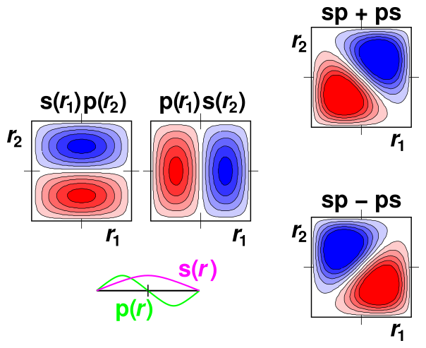
Classically, a two-particle problem involves two functions of one variable each. In contrast, QM generally requires us to describe this problem as a single function of two variables. So for two variables in three-dimensional space, the wavefunction has a six-dimensional abscissa, which is rather hard to visualize. However, the optical behavior of a dye molecule can be described (to a good approximation) in terms of electrons moving one-dimensionally along a tiny molecular “wire”. Let r1 be the r-coordinate of the first electron, and let r2 be the r-coordinate of the other electron. Then we can portray the wavefunction as a contour plot, as a function of the two variables r1 and r2, as shown in figure 1.
In the lower left, we see the single-particle wavefunctions s(r) and p(r). These are sinusoidal, as expected for the lowest modes of a one-dimensional particle-in-a-box system. This is plotted with the r variable running east/west, and the wavefunction ordinate running north/south.
Above that, we see the two-particle basis functions s(r1) p(r2) and p(r1) s(r2). These are plotted with r1 running east/west and r2 running north/south, while the wavefunction ordinate is shown in the third dimension – perpendicular to the paper – as a contour plot. Red indicates negative values, while blue indicates positive values.
Finally, in the right column, we see the gerade and ungerade combinations of the basis functions.
Along the diagonal where r1 equals r2, the probability vanishes for the ungerade combination ... but not for the gerade combination. Remember that the Coulomb energy goes line 1/|r1−r2|, so probability at or near the r1=r2 line counts for a lot. Therefore the Coulomb energy will be dramatically lower for the ungerade combination.
Note the following distinction:
| The contour plots in figure 1 depict Hilbert space. The variables r1 and r2 are independent variables in Hilbert space. They are depicted by perpendicular axes in the diagrams. | In real space (as opposed to Hilbert space), r1 is the r-coordinate of one electron, while r2 is the r-coordinate of the other electron. There is only one r direction, so in real space you cannot consider r1 to be perpendicular to r2; they are just two copies of the same r axis. The two symbols are different because they refer to different electrons. |
So far, we have explained why a spatial wavefunction that is antisymmetric with respect to exchange of electrons will have lower energy than one that is symmetric.
To derive Hund’s Multiplicity Rule, we need to connect this spatial symmetry with the spin multiplicity. By way of preview, the connection will hinge on the following propositions:
As an almost-corollary, the states of interest will have definite parity, i.e. either even or odd parity. States of indefinite parity would almost certainly be nonstationary.
Combining these two propositions, we see that symmetric spin arrangements will be associated with antisymmetric spatial arrangements, and will therefore have lower energy.
Disclaimer #1: Consider the contrast:
| Hund’s rules are traditionally applied to atoms. | This document applies to molecules. |
| The atom has a central potential. There is a nucleus at r=0 and not at r=1. | For a dye molecule, we approximate the potential as a square well, such that r=0 is a mirror image of r=1. |
| In an atom, you need to worry about screening. One electron screens the nucleus, so the other electron sees less effective nuclear charge. | For the dye molecule, screening is not high on the list of things to worry about. |
Disclaimer #2: Figure 1 correctly describes a particle in an ideal box, in particular a simple box with a flat floor and tall vertical sides. In a real dye molecule, things are much more complex. The “box” is made of a few atoms, and therefore has a very uneven floor. There will be a few very deep pits in the floor, located where the atomic cores are. That means that in addition to the electron/electron electrostatic interaction which you can estimate from figure 1, there will also be electron/nucleus interactions that must be taken into account. See reference 2 for details.
By way of background, consider the fundamental rule about identical particles. Baym (reference 5, page 391) expresses it like this:
Now it is an experimental fact that a pair of identical particles will always be found to have a wave function that is also an eigenstate of [the permutation operator] P21, and furthermore the eigenvalue, +-1, depends only on the kind of particles involved! ....Particles that must have symmetric states are called bosons .... Particles whose states must be antisymmetric are called fermions.
This is not really the best way to state the rule. This version cannot be taken toooo literally, for reasons Baym discusses on page 393. Even so, this version is good enough for present purposes.
Consider an atom such as hydrogen. We can describe it in terms of the atomic orbitals (s, p, d, f, etc.), which are well-known functions that you can look up in your chemistry books. Actually, though, what I’m really interested in is a dye molecule, which (as an initial approximation) can be modeled as a particles-in-a-box problem, in one dimension ... which makes things even simpler. In one dimension, the orbitals of interest for the dye molecule (in the independent-electron approximation) are:
| (1) |
where the box extends from -L/2 to +L/2. Actually, for most of what follows, all we need to know is that s() and d() are even functions, while p() and f() are odd functions.
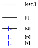
Within the independent-electron approximation, the Nth energy level for a particle in a box is proportional to N2. The ground state (S0) can be diagrammed as:
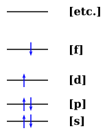
We can also draw things like the following, i.e. examples of low-lying singlet and triplet excited states:
Or
It is observed as a trustworthy rule that the triplet excited state (T1) always has a lower energy than the singlet excited state (S1). The question is: How can we explain this? How sure are we that this will always be the case?
In the context of the ground state of atoms, this rule is known as Hund’s Multiplicity Rule. It wasn’t immediately obvious to me that the corresponding rule would be valid in one dimension (instead of three), or valid for excited states (as opposed to ground states), let alone valid for molecules (as opposed to single atoms).
So (gasp!) I had to actually understand where the rule was coming from.
We can write the ground state as
| (2) |
where ↑ and ↓ refer to spin up and spin down, respectively; for example ↓1 means electron #1 is in the down state. Similarly r1 denotes the position of electron #1. Equation 2 satisfies the fermionic exchange rule quoted at the beginning of section 3, as you can verify by exchanging 1 ↔ 2 everywhere on the RHS, and observing that the sign of the wavefunction is flipped. We note in passing that this wavefunction is a state of definite parity (even parity), as you can verify by replacing r with −r everywhere on the RHS, and observing that the wavefunction is unchanged. Also, I will blow off all normalization constants – restoring the requisite factors of √2 is left as an exercise for the reader.
We can write the singlet excited state as
| (3) |
which also satisfies the fermionic exchange rule. The LHS has odd parity, as does each of the four terms on the RHS.
We can write one of the possible triplet excited states as:
| (4) |
which again satisfies the fermionic exchange rule. The LHS has odd parity, as does each of the four terms on the RHS.
In the independent-electron approximation d(r) would be identical to d′(r), and f(r) would be identical to f′(r), but I’m keeping them distinct so we can talk about electron-electron interactions if we want to.
Now the wacky thing, and a rather crucial point, is that we can construct another state by keeping just terms [a] and [d] from the RHS of equation 3. We can construct yet another by keeping just terms [b] and [c] from that equation. The same goes for the [a]+[d] terms the [b]+[c] terms in equation 4. Each of these pairs constitutes a subspace, closed under exchange. This gives us states such as:
|
The nice property of the four-term expressions equation 3 and/or equation 4 is that they have definite symmetry under exchange of the spatial part of the wavefunction separately, and also under exchange of the spin part separately. On the other hand, there is no law that requires wavefunctions to have any such separate symmetries.
A good way to see what is going on is to note that in the independent-electron approximation, we can form two-term states by superposing S1 and T1:
| (6) |
| (7) |
In the independent-electron approximation, there is a manifold of states all with the same energy. This includes the T1, S1, |A>, and |B>. Each of these states makes as much sense as any of the others.
Things get even more complicated when you consider other members of the T1 multiplet, which (in zero applied field) are part of the same degenerate manifold. We get lots and lots of states, all with the same energy.
However, when we (finally!) account for electron-electron interactions,
Nonstationary states are perfectly legitimate states. Sometimes, though, they are a bit hard to produce: For example, in the dye molecule there is a selection rule that favors the S0–S1 transition at the expense of the S0-T1 transition ... so it will be hard to go from the ground state to the sort of 50/50 superposition called for in equation 5c and equation 5d.
Now we can see the basis of Hund’s Multiplicity Rule. Recall equation 3 and equation 4:
| S1 = [ d(r1) f(r2) + d(r2) f(r1) ] · (spin part) (8) |
| T1 = [ d(r1) f(r2) − d(r2) f(r1) ] · (spin part) (9) |
and consider what happens when r1 is equal (or nearly equal) to r2. The T1 wavefunction vanishes for small Δ r, while the S1 wavefunction does not ... where we have defined Δ r := r1 − r2. So S1 will have a higher energy than T1, because of the Coulomb interaction ... as discussed in more detail in section 2.
One way to think about this argument is as follows:
The perturbation is likely to be rather large.
Another sidelight, and a bit of advice: Don’t forget the primes on the RHS of equation equation 4. You can’t build atoms or molecules just by writing down "the" orbitals and then filling them with electrons, the way you stick eggs into an egg-carton. The wavefunction for the Nth electron is heavily perturbed by the presence of the other N−1 electrons. You can usually tell by the symmetry that f′() is related to f(), but they are not the same in detail.
If you just look at the two-term states |A> and |B> as defined in equation 5a and equation 5b, you can easily convince yourself (by symmetry!) that they, to first order, not shifted either way by the electron-electron interaction. That is, narrowly speaking, true ... but highly misleading, because it overlooks the key lesson of degenerate perturbation theory: Since |A> is degenerate with |B>, you don’t have to shift |A> or shift |B> per se. Instead, the system can pivot to form linear combinations of |A> and |B>, and then shift one combination relative to the other. If the system can pivot, it will, in order to find the combination that is most sensitive to the perturbation.
This is the answer to a question that really bugged me when I was a student: Why do chemists tend to assume that every atomic wavefunction will separate into a space part and a spin part, each with a simple symmetry or antisymmetry (such as singlet, triplet, etc.)? Many people who ought to know better act as if this were an axiom of quantum mechanics, but of course it is not. It is not even true in general ... although it is a good approximation in a wide range of practical situations. It is what you get when you start with independent-electron wavefunctions, and then split the degeneracies via electron-electron Coulomb interactions, neglect all other interactions and perturbations, and then look for stationary states.
Other states certainly exist, but most of them won’t be stationary in situations where electron-electron Coulomb interactions are dominant.
It is fun to contrast the one-dimensional case (dye molecule excited states) with the three-dimensional case (Hund’s rule for atomic ground states). The fact that the triplet has lower energy in both cases tells us that the result – Hund’s rule – is rather robust, depending mainly on symmetry, stationarity, and the Coulomb interaction.