|
| |
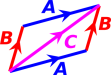
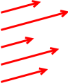
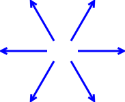
| Figure 1: Vectors with All the Same Direction | Figure 2: Vectors with All the Same Magnitude | |
This document reviews the fundamentals of what we mean by “vector”. It is more of a review than an introduction or tutorial. It tries to avoid some of the misconceptions that often creep into unsophisticated discussions of vectors.
A vector is something with direction and magnitude. This is the “grade school” definition of a vector, but it’s true, important, reliable, and actually quite sophisticated.
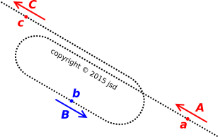
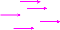
Informally, a vector can be represented as an arrow. For example, in figure 1, all the vectors have the same direction (but different magnitudes). Meanwhile, in figure 2, all the vectors have the same magnitude (but different directions).
Here’s a real-world example: velocity is a vector, because it has both a direction and a magnitude. Both the magnitude and the direction are important. Consider the contrast, as shown in figure 3:
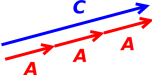
One thing that a vector does not have is a location. All of the arrows in figure 4 represent the exact same vector, because they all have the same magnitude and direction.
Similarly, back in figure 3, velocity vector A and velocity vector C are exactly equal, because they have the same direction and magitude. When we compare point C to point A, the time is different and the object’s position is different ... but the velocity doesn’t care about any of that. The two velocity vectors (shown in red) are equal.
For this reason, representing a vector by an arrow is imperfect and informal. A vector must not be «defined» in terms of the arrow, because the arrow has properties that the vector does not, including location. For more on this, see section 16.1.
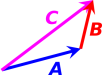
In any particular vector space, the vectors can be added. This is one of the defining properties of vectors (reference 1). You add them “tip to tail” as shown in figure 5.
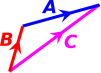
Addition is commutative, which means you can add the vectors in the reverse order, as shown in figure 6.
Tangential remark: When drawing vectors, the length of the arrow indicates the magnitude of the vector; meanwhile the orientation of the arrow, with help from the arrowhead, indicates the direction. That’s all that is required. In particular, there is nothing that requires the arrowhead to be at the end of the arrow. You can put the arrowhead somewhere in the middle of the arrow, as we see in figure 6. I mention this because with some drawing programs, it is relatively easy to construct a line with exactly the right length, but remarkably difficult to draw an arrowhead at the end without messing up the length. Even with the best drawing tools, a bunch of overlapping arrowheads tend to make the diagram look cluttered. So, especially when you are trying to do accurate arithmetic, as in figure 6, you might want to move the arrowhead to the middle.
You can combine figure 6 and figure 6 to form figure 7. For obvious reasons, this is called the parallelogram rule. It doesn’t tell us anything we didn’t already know. The parallelogram rule is just two copies of the tip-to-tail rule.
In any situation where C = A + B, we know just by re-arranging the algebra that A = C − B, B = C − A.
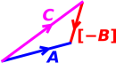
We can also subtract vectors using geometry directly. As always, the rule is: If you want to subtract B, add the opposite of B. (This is the axiomatic definition of subtraction!) So to find C − B, start at the starting point of C. Then add [−B], i.e. the opposite of B, always adding tip-to-tail. The ending point is the end of [−B]. This is shown in figure 8.
Another defining property is that you can multiply vectors by scalars, as shown in figure 9. You can also divide by scalars, using the simple rule: if A = sB then B = A/s, for any vectors A and B, and any nonzero scalar s.
Scalar multiplication distributes over vector addition: s(A + B) = sA + sB.
Remember that vectors are not numbers. Therefore this distributive law for vectors cannot be derived as a consequence of the familiar distributive law for ordinary numbers. It is a separate law.
It is guaranteed to be true because it is part of the definition of what we mean by vector. It is one of the vector-space axioms; see section 11.
We can compare directions as follows, for vectors with nonzero length:
If a vector has zero length, its direction is undefined, undefineable, and irrelevant.
In simple cases, the vector space has a dot product that allows us to quantify the magnitude of a vector, and quantify the angle between two vectors.
Beware that this is not the general case. There are important situations (e.g. thermodynamics) where there is no dot product. Roughly speaking, in such a situation we can draw vectors, but we don’t have a ruler to measure magnitude, and we don’t have a protractor to measure angles. As always, the vectors have direction and magnitude, but without a dot product, our notion of direction and magnitude is very weak and very restricted. We can always detect whether two vectors have the same direction or not, and if they have the same direction we can detect whether they have the same magnitude or not, but beyond that we cannot quantify direction or magnitude.
In the rest of this section, we restrict attention to situations where there is a dot product.
When we form the dot product of two vectors, the result is a scalar. (This is part of the axiomatic definition of dot product.)
We can use the dot product to quantify the magnitude of a vector:
| (1) |
Terminology: The magnitude of a vector is also known as the norm of the vector. In particular |A| can be called the norm of A, and |A|2 can be called the norm-squared of A.
We can also use the dot product to quantify the angle between any two nonzero vectors:
| (2) |
You can verify that the angle is independent of magnitude. For example, the angle between A and B is the same as the angle between A and 2B, which makes sense.
The vector-space axioms require the dot product to distribute over vector addition:
| (3) |
The axioms also require the dot product to be bilinear. That is, for any scalars λ and µ, we have:
| (4) |
Note that the bilinear property is consistent with the definition of magnitude (equation 1). You can easily prove that
| (5) |
which makes sense. On the LHS, we multiply the vector by a scalar, and then compute the magnitude. On the RHS, we first compute the magnitude, which gives us a scalar, and then multiply that scalar by another. In other words, multiplying vectors by scalars is consistent with multplying scalars by scalars.
As an amusing exercise, you can verify by direct calculation that
| (6) |
where θ is the angle between the two vectors. Note that this expression includes the Pythagorean theorem as a special case. You should verify that the equation make sense in the case where A = B, and where A = −B, and where A is perpendicular to B.
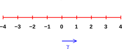
Here is a recipe for constructing a number line:
Pick some nonzero vector B. Compute the corresponding unit vector:
| (7) |
Then for any scalar s, you can construct a vector that “corresponds” to s by multiplying the vector b by this scalar:
| (8) |
Conversely, for any vector V in 1D, you can construct a scalar that in some sense “corresponds” to V by forming the dot product, namely:
| (9) |
In a 1D vector space this is a one-to-one correspondence, since:
|
As a corollary of equation 10b, you can show that |s| = |V|, in a 1D vector space. On the LHS of this expression we have the simple absolute value of a scalar, while on the RHS we have the magnitude of a vector. Beware that this is only a rather weak corollary, not a one-to-one correspondence, because there are four possibilities: |±s| = |±V|
In a multi-dimensional vector space, equation 10b turns into this:
| (11) |
where x̂ is a unit vector in the x direction. The term (V·x̂) x̂ is the projection of V onto the x direction. Equivalently we say (V·x̂) x̂ is the projection of V onto the one-dimensional subspace defined by x̂. It is not equal to V, except in the special case where V was already parallel to b.
Such expansions are so common that there is a special notation:
| (12) |
Terminology: x̂ is called a basis vector and Vx is called a mel. (In formal linear algebra, they are called matrix elements, but we don’t need to bother with that.)
Here’s a useful mnemonic: You can think of mel as short for meélange, meaning mixture. In equation 12, the mels tell us how much of each basis vector we need to mell together to reconstruct the vector V. Note that “mell” is a perfectly good English word meaning to mix or blend.
Note that the list of mels “corresponding” to a given vector V depends not just on V, but also on the choice of basis. If you pick a basis vector that points to the northeast, you get a number line where the mels increase to the northeast ... whereas if you pick a basis vector that points in the opposite direction, you get a number line where the mels increase to the southwest.
Because the choice of basis is arbitrary, no physically-significant answer (or physically-significant question) can ever depend on the basis or on the mels. Keep in mind that the mels are only a representation of the vectors, and indeed only part of a representation; do not think of them as “being” the vectors.
Consider the contrast:
| Vector | Mels |
| A vector exists as a physical and mathematical entity unto itself, independent of whatever representation (if any!) you choose. In general, try to do as much as you can using the vectors themselves. A great many theoretical results can be derived quite nicely without going anywhere near any basis or any mels; see e.g. equation 6. | There are some situations where it is expedient to convert vectors to the corresponding numbers, perform arithmetic on the numbers, and then convert back. In particular, simple calculators and spreadsheets are better at dealing with numbers than with abstract vectors. However, you should think of this as a slightly dirty trick. |
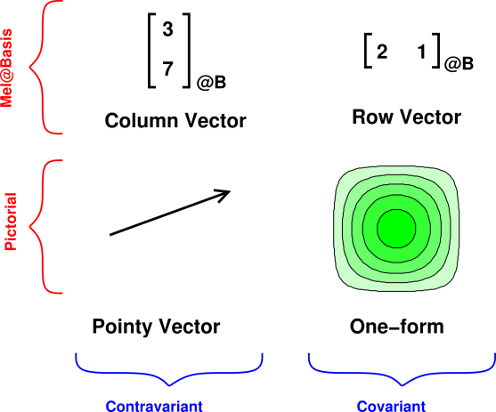
As can be seen in the two columns in figure 10, we can classify vectors as being contravariant versus covariant. This is an important, intrinsic distinction. It tells us something about the physical significance of the vectors. However, we defer until section 13 the discussion of contravariant versus covariant.
In this section we focus mainly on the question of representation, i.e. the row-to-row distinction in figure 10.
We can represent vectors using a pictorial representation (as in the bottom row of figure 10).
We can also represent vectors numericallly, in terms of mels, as in the top row of figure 10, or equivalently in equation 12. Changing the representation does not change the meaning of the vector.
It must be emphasized that in order to represent a physical vector in terms of mels, you need not only the array of mels but also the associated basis.
It is a remarkable fact that when working with vectors, certain mathematical operations can be carried out by working with the mels instead of the vectors themselves. For example, the following equation expresses multiplying a vector by a scalar and then adding another vector:
| (13) |
where we have expanded each of the vectors (P, Q, and R) in terms of its mels in a particular basis. This is guaranteed to work, because the operation of expanding a vector in terms of its components in a particular basis is a linear operation.
The remarkable thing is that you can carry out the calculation in equation 13 without knowing the details of the basis. The basis vectors just go along for the ride. You need the basis vectors if you want to know the physical significance of the equation, but in this situation you can do the arithmetic without knowing the physical significance. Just grind out the multiplications and additions: 2(1) + 5 = 7 and 2(−2) + 3 = −1.
Therefore, it is possible to drop the “@B” specifiers from equation 13 and still have a mathematically-correct equation. Provided the arrays uphold the vector-space axioms, it is OK to say that the arrays themselves are vectors, even if we cannot assign any physical significance to them.
On the other hand, you have to be careful, because there are plenty of other situations where it would not be safe to drop the basis specifiers. See e.g. equation 23.
What’s worse, horrendous confusion arises from the fact that some computer languages throw around the word “vector” with a meaning quite different from the physics meaning. They apply it to lists of numbers, and to lists of non-numerical objects, even when the lists do not uphold the vector-space axioms. In math and physics, such a thing would be called a list, array, or sequence.
The things we have been calling physical vectors could also be called mathematical vectors or topological vectors. It is tempting to call them geometric vectors but that is not quite right, because as discussed in section 13 there are important physical situations where we have a topology but don’t have a geometry. Some (but not all) of the things you would like to do with vectors can be done using only topology, without geometry.
A topological vector is an object P that lives in some space, possibly ordinary three-dimensional position-space, or possibly some more abstract space. The topological vector has direct, inherent significance in that space. Topological vectors can be diagrammed as arrows or by contours, without reference to any basis, as shown in the lower row in figure 10.
Pointy vectors can be added using the tip-to-tail rule. A similarly direct, graphical rule can be used to add one-forms.
There is no unique way to expand a topological vector in terms of its components. That is, without some nontrivial additional information, we cannot assign any physical significance to an expression of the form
| P = | ⎡ ⎢ ⎣ |
| ⎤ ⎥ ⎦ | (?allegedly?) (14) |
because we don’t know which observer’s basis is to be used. It makes incomparably more sense to write:
| P = | ⎡ ⎢ ⎣ |
| ⎤ ⎥ ⎦ |
| (15) |
which means
| P = a ex(@M) + b ey(@M) (16) |
where ex(@M) and ey(@M) are the basis vectors in Moe’s frame. The interesting thing is that we can equally well express P as:
| P = | ⎡ ⎢ ⎣ |
| ⎤ ⎥ ⎦ |
| (17) |
which means
| P = p ex(@J) + q ey(@J) (18) |
where ex(@J) and ey(@J) are the basis vectors in Joe’s frame. Note that all four of these expressions (equation 15) through equation 18) are simultaneously valid descriptions of the same topological vector P, since a ex(@M) + b ey(@M) = p ex(@J) + q ey(@J).
Beware: The notation here is inelegant and potentially confusing. Note the contrast:
| When talking about basis vectors, ex is a vector unto itself. It is the basis vector in the x direction. | In equation 22, P is a vector and P1 is one of its mels. P1 is not a vector. |
If you wanted to, you could think of e as some sort of higher-rank object, as a vector of vectors, so that the vector ex is a component of this higher-rank object. This is logical, but requires a bit of sophistication. For now, especially in an introductory course, it is simpler to say that the subscript x is just part of the name of the vector ex.
To repeat: When we are talking about the basis vector ex, the subscript x is part of the name of the vector, and indicates which member of the basis set we are talking about, namely the basis vector in the x-direction. The ex vector has components of its own; its x-component can be written as (ex)x.
Sometimes people try to alleviate this problem by choosing different names for the basis vectors. One choice is to use {i, j, k} instead of {ex, ey, ez}. Some people like to decorate unit vectors by writing a hat over them, as in {î, ĵ, k̂}. Another version of this is {x̂, ŷ, ẑ}. To summarize:
| (19) |
However, I don’t recommend any of the substitutions in equation 19, for reasons to be discussed below. The {ex, ey, ez} notation is better. However, there is one improvement we can make: We can use numbers (rather than letters) to identify the coordinates, and then use corresponding numbers to identify the basis vectors. That is: the coordinates names {x1, x2, x3} turn out to be more practical than {ex, ey, ez}. The correspondence is:
| (20) |
The basis vectors are numbered accordingly. Also, in the Clifford-algebra literature, basis vectors are commonly denoted by γ rather than e. That is,
| (21) |
In equation 21, all three options for naming unit vectors have the same potential to cause confusion, because e1 looks like a 1-component just as much as ex looks like an x-component. Using γ instead of e isn’t a fundamental change, but reduces the conflict with other uses of the symbol e. For the rest of this document, we will use γ.
The practice of using subscripts to denote which basis vector is well established in the math and physics community and is unlikely to change anytime soon The obvious disadvantage is that is a never-ending source of confusion for students. The practice does however have some significant advantages, such as allowing expressions such as equation 16 to be written more compactly:
| (22) |
where the last line uses the Einstein summation convention, i.e. implied summation over repeated indices.
When working with vectors, often you can calculate everything you need to know without ever using a basis. On the other hand, sometimes it helps to have a basis.
You get to choose the basis. Sometimes one particular basis is obviously convenient, but sometimes there are lots of possibilities.
Any complete set of orthonormal vectors can be used as a basis. You can choose any basis set you like (but keep in mind that other folks may choose differently).
Beginners should choose one basis and stick with it until the end of the calculation. If the initially-chosen basis turns out to be inconvenient, restart the calculation from the beginning using a better basis, and use the new basis consistently throughout.
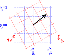
In more advanced settings, it may be convenient to do part of the calculation in one basis, and part in another. A rough idea of how this works is shown in In figure 11.
Joe’s reference frame is shown in blue, while Moe’s reference frame is shown in red. The topological vector P is shown by the heavy black arrow. It does not “belong” to either frame; it is a real topological object with its own independent existence. Joe looks at P from one viewpoint, while Moe looks at it from another viewpoint.
The crucial point is that P is not changed when we switch from one reference frame to another. The topological vector neither knows nor cares who – if anyone – is looking at it.
Similarly, if we have a vector relationship such as P = Q + R, we can add the vectors A and R graphically, tip to tail, without reference to any coordinate system. All observers agree that P is the sum of Q and R ... even if they do not agree about the x-components, y-components, et cetera.
If we choose to expand the vector P in terms of components, as in equation 23, we find that a is not numerically equal to p, and b is not numerically equal to q. Nevertheless, equation 23 is in fact an equation, expressing the equality of two topological vectors:
| ⎡ ⎢ ⎣ |
| ⎤ ⎥ ⎦ |
| = | ⎡ ⎢ ⎣ |
| ⎤ ⎥ ⎦ |
| (23) |
Metaphorically speaking, this is like writing 2·12 = 3·8 ... it’s two expressions for the same thing. More precisely, the meaning of equation 23 is explained above; see equation 15 and equation 17.
Note that it would be a mistake to leave off the “@Moe” and “@Joe” specifiers from equation 23. That would leave us with a false equation:
| ☠ | ⎡ ⎢ ⎣ |
| ⎤ ⎥ ⎦ | = | ⎡ ⎢ ⎣ |
| ⎤ ⎥ ⎦ | ☠ (24) |
By convention, in an equation such as equation 24, if no basis is specified it is implied that the basis is the same on both sides of the equation. As another way of saying the same thing, two arrays (as in equation 24) are equal if-and-only if the corresponding components are equal.
In this case they cannot be equal. That is to say, if equation 23 is true, then equation 24 must be false. You can easily prove this by using figure 11 to graphically evaluate p and q (the projections of the vector onto Joe’s axes) versus a and b (the projections of the vector onto Moe’s axes). You can also infer this by comparing equation 16 to equation 18.
All the fundamental laws of physics are independent of the choice of basis. That means it is possible (and indeed common) for the basis vectors to have no direct physical significance. Sometimes it is convenient to choose basis vectors that are related to the physically-relevant vectors, but this is by no means necessary.
If you see a law that seems to depend on the choice of basis, you should find a better way of expressing the law.
In some situations there may be a “conventional” basis, but the conventions are definitely context-dependent; they vary from situation to situation.
Note that all three of the foregoing examples are right-handed systems.
Note that when describing directions on paper, even when the paper is lying on a table, it is conventional to speak of the “vertical” direction as if the paper were hanging on a wall. This conflicts with almost all other uses of the word “vertical”, but that’s how it is.
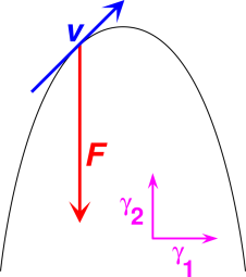
Suppose we are interested in some force F and some velocity v. We choose to expand these in terms of some basis vectors {γ1, γ2}, so that
| (25) |
Note that F is a vector, whereas the mels F1 and F2 are scalars.
We can apply this expansion to the physical situation shown in figure 12. We observe that v1 is positive, v2 is positive, F1 is zero, and F2 is negative in this situation.
In this example, we have spelled things out in enough detail that there is no doubt as to the correct interpretation. So this counts as a good example.
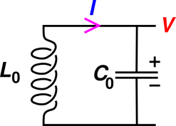
Now let’s consider a contrasting example, based on figure 13. The variable I represents the current. In this diagram, the magenta arrowhead must be considered a basis vector. Suppose we calculate that at the moment of interest, the value of I is negative. This means that the physical current is flowing in the direction opposite to the magenta arrowhead.
Note the contrast:
| In figure 13, a negative I-value means the current is flowing in the direction opposite to the arrowhead. | In figure 12, a negative F2-value does not mean that the force is opposite to the red F vector. It just means that the force vector is opposite to the γ2 vector. |
It is not particularly obvious from looking at figure 13 that the magenta arrowhead is mean to represent a basis vector, not the physical current. See section 7.3 for more on this.
This is a perennial source of confusion. Part of the problem is that the current is constrained to move in one dimension, along the wire. The same problem arises in mechanics, when we consider one-dimensional motion. In one dimension, there is a one-to-one correspondence between vectors and scalars, and sometimes people get sloppy about the distinction between F (the vector) and F1 (the mel). Figure 13 is an example of sloppy usage. The variable I is a scalar. Presumably it represents the mel. If you want to think of the current as a vector with direction and magnitude, you have to multiply I by the basis vector. Alas, there is not any conventional symbol for representing this vector, so far as I know.
You might think that the situation would be even more confusing in higher-dimensional spaces, but ironically it’s actually less confusing. That’s because when there are two or more dimensions, it’s more obvious what’s a vector and what’s a scalar.
One should never talk about vectors as being “positive” or “negative”. It’s a bad practice in a one-dimensional space, and an outright impossibility in a higher-dimensional space. That’s because “positive” means greater than zero, and there cannot be any “greater-than” relationship when D>1. Even in one dimension, it is good practice to talk about vectors in terms of magnitude and direction, rather than positive and negative. If the basis vector is rightward and the physical vector is leftward, say that it is leftward; don’t say it is negative. The notion of positive and negative should be restricted to scalars only. Given a vector F in two or more dimensions,1 you can say that one of its mels such as F1 is positive or negative, but the whole vector F can never be positive or negative.
In any case, remember that in figure 12, the physical vector F exists independently of whatever basis (if any) you choose to use.
Constructive suggestion: Whenever possible, label your vectors so as to make it clear what is a basis vector and what is not, as we have done in figure 12. See section 12 for some related suggestions.
When I started graduate school, the very first homework assignment involved a vector pointing to the left. Every first-year student diagrammed it as an arrow pointing to the left, and quantified it as a negative number. The grader (a third-year grad student) marked every student wrong.
Some of us got out our torches and pitchforks and marched to the grader’s office to explain a few things, as shown in figure 14.
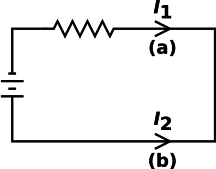
Consider the simple circuit shown in figure 15.
In a fundamental sense, “the” current is the same everywhere in the circuit, yet numerically I2 is the negative of I1.
The smart way to deal with this is to recognize that “the” current is a one-dimensional vector!
This comes as a shock to some people, but really I’m just giving a name to a widespread, conventional, tremendously useful practice. The first crucial application is to say that the symbol “–>–’ is a basis vector while numbers such as I1 and I2 are not vectors, but merely mels. This allows us to write an expression in terms of mels: 2
| (26) |
In contrast, we can also write an expression in terms of vectors:
| (27) |
where as before, [⋯]@F is my favorite notation for expressing a vector in terms of its mels relative to the specified basis F.
As always, there is an isomorphism between one-dimensional vectors and plain old scalars, but isomorphic is not the same as indistinguishable. The crucial distinction here is that vectors can be expanded in terms of a chosen basis, while scalars cannot. This is crucial because different people can choose different bases.
The following may make you feel better about the fundamental physics: An electron moving through space has a velocity, and the velocity is a vector. If we confine the electron to a wire, the average velocity is constrained to be parallel (or anti-parallel!) to the wire ... but it is still a vector. If velocity is a vector, then current must be a vector.
The current in a wire is assumed to run along the wire, but that still leaves a question as to which of the two possible directions. It is a longstanding and necessary tradition that in circuit diagrams such as figure 15, we take I2 to be a scalar, and the corresponding physical current vector is I2 times a unit vector. The direction of the unit vector is indicated by an arrowhead. Introductory textbooks often disguise this issue because they can use 20/20 hindsight to arrange the arrowheads so that all (or nearly all) DC currents have positive components. However, in the real world of circuit analysis, even for DC circuits you often have to draw the diagram and define your variables before you know which way the current will be flowing … and for AC circuits talking about “the” direction of the current is pointless anyway.
To repeat: The arrowhead on the diagram does not say that the current flows in the direction of the arrowhead! If I2 is negative, the direction of current flow is opposite to the arrowhead. The arrowhead is just a basis vector, like the magenta vectors in figure 12. It may help to note that the arrowhead has no length associated with it; it’s just a disembodied arrowhead, not a complete arrow, so it cannot possibly represent the magnitude and direction of the actual current.
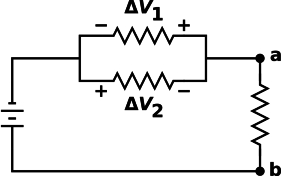
It should go without saying that the voltage drop ΔV is another one-dimensional vector. There are a couple of different conventions for diagramming the voltage basis vectors. These are shown in figure 16.
For the upper two resistors, the basis direction is indicated by the + and − signs. This allows us write3
| (28) |
Using another convention for the third resistor, we can write the voltage between points a and b as follows:
| (29) |
Vab is the negative of Vba, even though they are representing exactly the same physics. Purists might prefer to write this as ΔVab and ΔVba, but in practice, engineers don’t bother to write the deltas in situations like this, because the meaning is 100% clear already.
Note: This underscores the #1 rule of electrical engineering: Draw the circuit diagram. Without that, nobody knows what you’re talking about. It’s amazing how often callow students think they can solve the problem in their head, without drawing the diagram, in situations where super-smart professional engineers draw the diagram.
In any situation where there is only one reference frame being used, the distinction between arrays and topological vectors is not very important.
However, in many situations – in physics as well as life in general – it is important to be able to see things from more than one point of view. The technique of switching from one reference frame to another has been standard procedure in physics since at least the time of Galileo.
The fundamental laws of physics can be written as topological vector equations, valid in any reference frame, and indeed valid even if you don’t have any reference frame at all. Examples include the second law of motion and the Maxwell equations, which are conventionally represented in terms of 3-dimensional topological vectors, so that the representation is manifestly invariant with respect to arbitrary rotations in 3-dimensional space.
Tangential remark: With a bit of extra work, these laws can be re-expressed in terms of 4-dimensional topological vectors, making manifest their invariance with respect to arbitrary rotations in spacetime – including boosts – as discussed in reference 2 ... but if you don’t know what this remark means, don’t worry about it.
The best use of topological vectors and arrays is to use them together, leveraging one against the other. Topological vectors are particularly useful at the conceptual and strategic level, to set up the outline of the calculation and carry out the major steps. Every so often along the way, expanding the topological vector as an array of components in a chosen basis is useful for evaluating this-or-that subexpression. An amusing example of this combined approach can be found in reference 3.
It is important to think clearly about both topological vectors and arrays. Alas, the fact that people heretofore have used the same term – “vector” – to refer to two different concepts makes it hard to think clearly about either one.
Students’ proficiency with topological vectors seems to be a regrettably non-monotonic function of their overall sophistication:
The problem is that all too commonly, their knowledge of arrays of numerical elements interferes with and detracts from their understanding of topological vectors. The mels get improperly separated from their basis.
The thing we have been calling a topological vector is properly called a tensor; all our examples have been rank=1 tensors. Similarly, the thing we have been calling an array is properly called a matrix; all our examples have been rank=1 matrices, i.e. columnar matrices with N elements (as opposed to the more common square matrices with N×N elements). Therefore in an array of mels, the mels could also be called matrix elements. In this document we call them simply mels.
Tensors exist as geometric objects unto themselves, independent of their representation in terms of matrices in this-or-that basis. Tensors can be represented by matrices in much the same way as numbers can be represented by numerals.
We postponed calling topological vectors and arrays by their proper names (tensors and matrices) for pedagogical reasons. As the saying goes, learning proceeds from the known to the unknown. The important ideas in this paper do not require any prior knowledge of tensors or matrices.
Vectors in one dimension are a special case, because there is an isomorphism between the vectors and the scalars.
This causes problems in an introductory physics class, because the usual practice is to introduce vectors in connection with one-dimensional motion. It makes sense to keep things as simple as possible, hence D=1. On the other horn of the dilemma, it makes sense to develop good habits and avoid bad habits that will have to be unlearned later.
Suggestion: Avoid writing equations of the form
| (30) |
and especially avoid
| (31) |
because the LHS of these equations is a vector while the RHS is a scalar. Also, in equation 31, the “>” operator only exists for scalars. In D=1, such equations are arguably technically acceptable, but they are pedagogically unsound, because they blur the distinction between vectors and scalars.
Constructive suggestion: Better alternatives exist.
You can use this to keep track of the distinction between vectors and scalars. For example it allows you to write
| (32) |
where we have dropped the arrow from v in accordance with the no-decoration policy explained in section 12.
It is useful to distinguish:
Beware that the word “component” is ambiguous. Depending on context, it can refer either to a mel or to a projection, as follows:
For any topological vector V, this means:
To avoid ambiguity, it may help to avoid the term “component” altogether; if you mean “mel” say “mel” (or perhaps “matrix element”), and if you mean “projection” say “projection”.
Projections have the nice property that we can take projections in any direction, not just along some pre-ordained set of basis directions. In general, the projection operator in the q-direction is
| Pq := |
| for any nonzero vector q (33) |
so that Pq(V) is the projection of V in the q-direction. This allows you to form projections in the direction of some q that is physically relevant to the problem. You don’t want to be restricted to a pre-ordained basis that typically has little or no physical significance.
As a rule, whenever you can formulate the problem topologically, using projections, you’re better off doing it that way, rather than introducing a basis and grinding out the mels.
The denominator in equation 33 ensures that the projection operator works properly for any nonzero q, not just for unit vectors.
Tangential remark: It is important to keep computers in their place. When simple computer programs work with vectors, they use numerical mels internally ... but so what? The physics is still in the arrows and contours, not in the mels. By way of analogy, computers do arithmetic using binary internally, but that doesn’t mean we humans should switch to using binary for everyday purposes. I’ve never seen a 110111 MPH speed-limit sign. (I keep expecting some smart-aleck student to make one, but it hasn’t happened yet.)
Some textbooks are better about this than others. Some of them define vectors as arrows ... but then lapse into a mel-based formalism soon as they start doing actual calculations, weakening the connection to the real physics.
If you are in a hurry, you can judge a textbook according to how it defines the dot product.
A second quick way of checking a text involves looking to see if the term “projection operator” is in the index. Alas I don’t know of any general-physics text that passes this test. (If anybody knows of one, please tell us about it.)
A more thorough check of the text involves looking at the end-of-chapter problems to see if they involve geometric relationships between vectors, as opposed to grinding out numerical mels.
The cleanest and classiest way I know to define the dot product is to postulate the existence of three vectors in space (or four vectors in spacetime) for which we know the dot products. It is not necessary to assume these vectors are orthonormal, but without loss of generality we will do so, for convenience.
We postulate the existence of at least one set of basis vectors with the following properties:
| (34) |
which just says the basis is orthonormal. In spacetime, we generalize equation 34 as follows:
| (35) |
but if you aren’t doing relativity you can ignore equation 35; don’t worry about it.
We do not assume there is only one basis. Given any such basis, you can construct innumerable other bases by taking linear combinations.
In any case, we postulate that the dot product is bilinear ... which is the same as saying there is a distributive law, such that “dot” distributes over “plus” as follows:
| (36) |
Given all that, you can calculate the dot product of any two vectors by expanding each vector in terms of the basis vectors in accordance with equation 16, redistributing the terms in accordance with equation 36, and then dotting the basis vectors using equation 34.
We can write any possible vector as a linear combination of the basis vectors. Then we can take the dot product of any vector by direct appeal to the axioms. In particular, as a corollary of this definition of dot product, suppose we have two spacelike vectors A and B that are known in terms of linear combinations of the basis vectors, namely
| (37) |
then their dot product is
| A · B = AxBx + AyBy + AzBz (spacelike) (38) |
as you can verify by direct substitution and turning the crank. We emphasize that equation 38 is not the definition of dot product; it is merely a corollary, valid under certain conditions. (The corresponding expression for spacetime vectors has a minus sign in it, not all plus signs.)
When we follow this approach, the dot product defines what we mean by angle. It also defines what we mean by length. This is important in abstract and/or unfamiliar spaces, where the notions of angle and length might not have been intuitively obvious. In particular, equation 34 has an elegant, simple, but very nontrivial extension to spacetime, as discussed in reference 2.
This approach (the axiomatic definition of dot product) reverses the idea in item (b), allowing us to define cos(θ) := A · B / |A| |B|.
As discussed in reference 4, a name is not the same as an explanation. Do not expect the structure of a name or symbol to tell you everything you need to know. Most of what you need to know belongs in the legend. The name or symbol should allow you to look up the explanation in the legend.
The convention of using boldface to represent vectors fails both in handwritten notes and in ASCII email. The convention of drawing an arrow atop the symbol fails in email.
The convention of using a decorated letter to represent a vector while the corresponding undecorated letter represents the magnitude of the vector is cute, but is not worth the trouble. If you want the magnitude of F, write |F| explicitly. The cost of writing |F| when you want the magnitude is infinitesimal compared to the cost of decorating F when you want the whole vector.
Perhaps most importantly: All schemes involving decorated vectors fail miserably in the context of Clifford algebra, aka geometric algebra, where some quantities have both a scalar piece and a vector piece. See reference 5. A rotor is an important example with a scalar piece and a bivector piece.
It is remarkable that the mathematical definition of “vector space” (as set forth in reference 1) does not include any mention of a dot product.
That means we can have vector spaces for which we have no notion of length and no notion of angle. An important physical example of this is thermodynamics. As discussed in reference 6, there is an abstract space – state space – where there are various “functions of state” including energy (E), entropy (S), enthalpy (H), pressure (P), temperature (T), volume (V), et cetera. The gradient vectors dE, dS, dH, dP, dT, dV, et cetera are well defined (usually if not always), but there is no way of knowing the angle between such vectors. (Occasionally somebody will assume that a certain pair of such vectors is orthogonal, but there is no advantage to making such an assumption. If you do the math right, any valid result that can be obtained with such an assumption can be obtained without it, in every case I’ve ever seen.)
Such vector spaces tend to come in pairs, pairing a space of pointy vectors with a space of one-forms. That’s a good thing, because either member of the pair by itself wouldn’t be very useful.
If you visualize a pointy vector as a little arrow with a “tip” and a “tail”, you absolutely should not visualize a 1-form the same way.
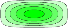
Suppose we want to visualize the gradient of some landscape. If you visualize the gradient as a pointy vector, it points uphill. In many cases, though, you are better off visualizing the gradient as a one-form, corresponding to contour lines that run across the slope.
You can judge the magnitude of the 1-form according to how closely packed the contour lines are. Closely-packed contours represent a large-magnitude 1-form. To say the same thing the other way, the spacing between contours is inversely related to the magnitude of the one-form.
Contour lines have the wonderful property that they behave properly under a change of coordinates: if you take a landscape such as the one in figure 10. and stretch it horizontally (keeping the altitudes the same) as shown in figure 18, the slopes become less. The contour lines on the corresponding topographic map spread out by the same stretch factor, as they should, to represent the lesser slope. In contrast, if you try to represent the gradient by pointy vectors, the representation is completely broken by a change in coordinates. As you stretch the map, the pointy vector doesn’t stretch; it has to get shorter to represent the lesser slope. If you want to represent a gradient, pointy vectors aren’t nearly so well-behaved as 1-forms; they aren’t attached to the real landscape the way contour lines are.
Of course, pointy vectors are needed also; they are appropriate for representing the location of one point relative to another in this landscape. These location vectors do stretch as they should when we stretch the map.
| pointy vector | one-form | |||
| Example: | distance | slope | ||
| Represented by: | column vector | row vector | ||
| When we stretch the map: | gets bigger | gets smaller | ||
| Adjective: | contravariant | covariant | ||
| Dirac notation: | ket |⋯⟩ | bra ⟨⋯| | ||
See reference 7 for more about Dirac bra-ket notation.
This may seem somewhat nitpicky ... but doing it right is just as easy as doing it wrong, so why not do it right?
Position is not a vector. A position is a zero-sized point. A position has neither direction nor magnitude.
The displacement vector from one position to another is a vector ... even though the positions themselves are not vectors.
You are not obliged to choose an origin, and your origin (if any) may be different from mine (if any). However, if you do choose an origin, you can establish a one-to-one correspondence between positions and vectors, namely radius vectors, by considering the displacement from the origin. However, this must be considered secondary, optional, and gauge-dependent. That is, it depends on the choice of origin, which is arbitrary.
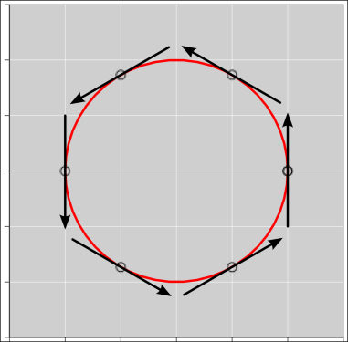
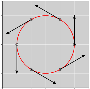
In figure 19 and similar diagrams, the following rules apply: The black arrows represent a vector field. For each arrow, the black circle tells which point in the field is being described by the vector. We call this the point of attachment. The length and orientation of the arrow tells us the magnitude and direction of the field at that point.
As emphasized in section 2.1, a vector has direction and magnitude, but it emphatically does not have a location. Therefore these diagrams need both an arrow and a small circle; the arrow represents the direction and magnitude, while the circle represents the location.
Suppose we wish to depict a divergence-free field, such as a magnetic field or the steady flow of a conserved fluid. There are several ways of doing this, some of which work better than others.
In figure 19, each vector is plotted in such a way that the point of attachment coincides with the midpoint of the arrow.
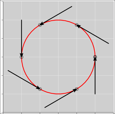
| For figure 20, the point of attachment coincides with the tail of the arrow. | For figure 21, the point of attachment coincides with the tip of the arrow. |
The contrast is worth emphasizing:
For most purposes, figure 19 is a much better depiction, insofar as it is easier to interpret correctly. Remember, we are trying to depict a divergence-free field. Figure 19 “looks” divergence-free. That is to say, it quite appropriately “looks” like the vector is just pulling you along a field line, with no tendency to pull you away from the field line.
Remember that a vector has a direction and magnitue but not a location. In diagrams such as these, you could perfectly well plot the arrow a couple of centimeters away from the point of attachment if you thought that would help. It would mean exactly the same thing.
As mentioned in section 2.2, a vector does not have a location. It has a direction and magnitude, and nothing more.
In physics, there are some physical situations where a full description requires more than a vector. For example, you might need to know both the force and torque.
As mentioned in section 2.2, when you draw an arrow it has a magnitude, direction, and position. Therefore the arrow is not an entirely faithful representation of a vector. To represent a vector, you musth use your imagination to detach the arrow from its location, so that only the direction and magnitude remain.
It is useful to deal with vectors as objects unto themselves, i.e. vectors with direction and magnitude. Vectors can be added tip-to-tail, without reference to components.
It is also useful sometimes to represent vectors in terms of components, and to work with arrays of numerical mels.
A valuable and easily-achievable goal is to be able to see things both ways. A skilled person should be able to switch from basis A to basis B to no basis at all and back again.
We should avoid the interference mentioned in item (b) in section 8. That is, we should teach people to use arrays of mels while deepening – not lessening – their understanding of topological vectors as real, physical objects that have meaning independent of their mels, independent of any basis, and independent of any observers.