1  An Example

Let’s talk about the process that can be used to acquire an understanding of the type Dirac was talking about. Let’s investigate an example, namely the following expression:

It must be emphasized that we care mostly about the process that will be used. We care more about the process than we care about this particular example. Expression 1 is moderately useful, but it is not nearly so useful as the general-purpose process of figuring things out.

1.    First bit of advice: If you are given an equation, ask where the equation came from. In this case, let’s assume the equation arose in connection with electrical resistors in parallel. (It could also have arisen in connection with capacitors in series, or lenses in series, or various other things.)

For present purposes, we restrict attention to the case where x and y are non-negative real numbers, which is appropriate for ordinary resistors. (The case of negative or complex x and y is also interesting, and is relevant for capacitors and inductors, but let’s leave that for another day.)

2.    Another bit of advice: Draw the picture. For example, if we are dealing with electronics, draw the circuit diagram. You’d be amazed how often callow students think they can get by without drawing the diagram, in cases where super-smart professional engineers do draw the diagram.

  

Figure 1: Resistors in Series and in Parallel

3.    Also: Whenever possible, write an equation, as opposed to a free-standing expression without any name and without any clear relationship to anything else. In other words, don’t do what I did in expression 1 above. Instead write something like

InvAd(x, y)   :=   1 1/x + 1/y

(2)

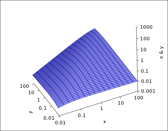
which defines InvAd as a function of two variables.

4.    Some more advice: As the famous philosopher D.N. Adams once said: Don’t Panic.

It may be that most of your experience has dealt with functions of one variable, such as sine, cosine, square root, et cetera. Now we have a function of two variables, which is somewhat harder to visualize ... but not unreasonably so, as we shall see.

5.    As a related point: You don’t need to figure out everything all at once. The first time you encounter the equation 2, you should think about it for a while, and work out some of the properties. Figure out some of the ways in which it is connected to other things you know.

Then, the next time you encounter it, think about it some more. Figure out some more of the properties. Figure out some more of the connections.

We call this the spiral approach. You begin by learning some bare facts. Then you spiral back and use principles to connect the dots. Then you learn some new facts and spiral back again to connect them to all the previously known facts and principles. And so on.

Here is a scenario that may not apply to you personally, but illustrates the sort of thing I am talking about.

• The first time you see equation 2, you might connect it only to the axioms of algebra, because that’s all you know.
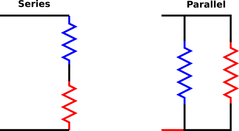
• The next time you see it, in the context of resistors in parallel, you can connect resistors to the equation and to the axioms.
• The next time you see it, you can relate capacitors in series to resistors in parallel and to the equation and to the axioms.
• The next time you see it, you can relate thin lenses to capacitors to resistors to equations to axioms.
• The next time you see it, you can relate De Morgan’s theorem to thin lenses to capacitors to resistors to equations to axioms.
• et cetera.

You may think this section presents more than enough details about the InvAdd function, but actually I have left out more than half of the story. There’s a lot more you can figure out if you want. See e.g. section 3.

6.    In equation 2, the name “InvAd” is something I just made up. It is short for “Inversely Add”. The point is, you are allowed to invent your own terminology, your own notation.

You can’t give something a clever name until after you know what it does. Therefore the first time you encounter something, give it a nondescript temporary name, such as F. After you figure out what it does, you can go back and rename it.

7.    It never hurts to do a few numerical examples, such as:

InvAd(1, 1)   =   1/2

(3)

8.    It would be nice to evaluate InvAd(0, 0), but the definition given in equation 2 is ill-behaved when x or y is zero. However, we can extend the definition as follows:

InvAdd(x, y)   =   0      when xy=0      (4a)   =   xy x + y      otherwise      (4b)

The RHS of equation 4b would be ill-behaved if we applied it when x=y=0, but we have nothing to lose by simply defining InvAdd(0,0) to be zero. This is the only reasonable answer, as you can see by setting x equal to y and then taking the limit as they both go to zero.

Equation 4 is equivalent to equation 2 whenever xy is nonzero ... and since equation 4 is well-behaved at zero and equation 2 is not, we have nothing to lose by studying the InvAdd function instead of the InvAd function. So let’s do that.

9.   

We can turn InvAdd into a function of one variable by holding the other variable constant. For example, we can evaluate:

In contrast:

InvAdd(0, y)   =   0       for any y      InvAdd(x, 0)   =   0       for any x              (5)

∞ + y   =   ∞       for any y      x + ∞   =   ∞       for any x              (6)

This makes sense in terms of the physics of a resistor in parallel with a dead short.

This makes sense in terms of the physics of a resistor in series with an open circuit.

10.   

Here is another way of turning InvAdd into a function of a single variable. You can show that:

In contrast:

InvAdd(∞, y)   =   y       for any y      InvAdd(x, ∞)   =   x       for any x              (7)

0 + y   =   y       for any y      x + 0   =   x       for any x              (8)

That tells us that an infinite resistance is the identity element for the InvAdd operator (resistors in parallel).

A zero resistance is the identity element for the addition operator (resistors in series).

Note that strictly speaking infinity is not a number and in general cannot safely be treated as a number ... but in this narrow context it is OK. A thin lens with infinite focal length is a well-known and harmless concept. Also, infinite resistance is a well-known concept. It can sometimes get you into trouble, e.g. if you hook a constant-current source to an infinite impedance load ... but that is no worse than hooking a constant-voltage source to a zero-impedance load.

11.   

Here’s yet another way of turning our function into a function of a single variable: We can use the same variable twice. That gives us:

In contrast:

InvAdd(x, x)   =   x/2        for any x              (9)

x + x   =   2x        for any x              (10)

In other words, InvAdd(x, x) is a straight line with slope 1/2. This has an obvious physical significance in terms of identical resistors in parallel.

In other words, sum(x, x) is a straight line with slope 2. This has an obvious physical significance in terms of identical resistors in series.

so we already understand a few things about this function.

12.    It is always good to think about scaling laws in general and dimensional analysis in particular. See reference 1 and reference 2.

In this case, we discover that when evaluating InvAdd(x, y), the two input variables need to have the same dimensions; otherwise the denominator in the definition (equation 4) doesn’t make sense.

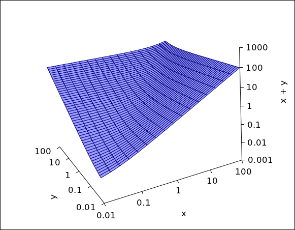
We also discover that the result returned by InvAdd(x, y) has the same dimensions as x and y. So in this way, InvAdd has something in common with the addition operator: InvAdd(x, y) has the same dimensions as sum(x, y).

13.    Let’s pay attention to the process used in the previous step. The learning process depends heavily on making connections. This has been understood quite explicitly for more than 100 years (reference 3) and understood to some degree for thousands of years (reference 4).

The recall process depends on using connections to fish up ideas when they are needed. Therefore the learning process depends on forming appropriate connections. This takes time and effort. Whenever you are exposed to a new idea, you need to mull it over. You need to ponder it, looking for ways in which it is similar – or dissimimlar – to previously-known ideas.

So, in item 12 as well as in item 11 establishing a connection between the InvAdd function and the sum function greatly strengthens our understanding of the InvAdd function ... and even strengthens our understanding of the sum function.

14.    We can immediately exploit this connection as follows: Since sum(x, y) is more conveniently represented using an operator, as x + y, we can define our own operator to represent InvAdd(x, y), namely the ∥ operator (pronounced “parallel”). We define it as:

x ∥ y   :=   InvAdd(x, y)            =   xy x + y

(11)

Again: You are allowed to define your own notation.

Learning is not a routine, mechanical process. It is a creative process. See reference 5.

15.    At this point, other analogies immediately suggest themselves. You can easily verify that

the commutative property:  x ∥ y   =   y ∥ x      (12a)      the associative property:  x ∥ y ∥ z   =   x ∥ (y ∥ z)      (12b)     =   (x ∥ y) ∥ z               a distributive property:  k (x ∥ y)   =   (kx) ∥ (ky)      (12c)

x + y   =   y + x      (13a)            x + y + z   =   x + (y + z)      (13b)     =   (x + y) + z                     k (x + y)   =   (kx) + (ky)      (13c)

All of these make sense in terms of the physics of resistors in parallel.

All of these make sense in terms of the physics of resistors in series.

Note that there is no such thing as “the” distributive property, because there are lots of different things that might or might not distribute over other things. Examples include:

• In ordinary arithmetic, multiplication distributes over addition, as in equation 13c.
• Multiplication distributes over InvAdd, as in equation 12c.
• As a counterexample, ordinary addition does not distribute over multiplication.
• In Boolean logic, BooleanAnd distributes over BooleanOr.
• Also in Boolean logic, BooleanOr distributes over BooleanAnd.

See also item 29 for a discussion of a generalized distributive law.

A remark about the process: Again we are making connections, connecting the algebraic properties of the ∥ operator to the physical properties of electronic circuits ... and also to the algebraic properties of the + operator. Obviously ∥ and + are not exactly identical. They are in some ways the same, and in other ways the opposite.

16.    Let’s change tactics now and examine the asymptotic behavior. In particular we compare the of InvAdd (resistors in parallel) to the asymptotic behavior of plain old addition (resistors in series).

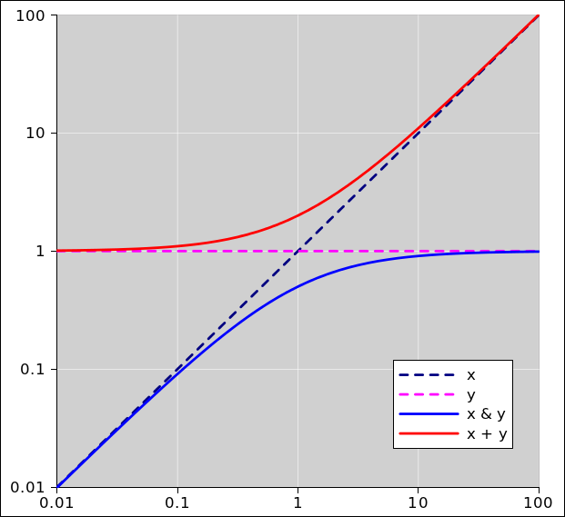
You can easily verify that if we hold y constant, then as x approaches zero,

x ∥ y   →   x              (14)

x + y   →   y              (15)

Similarly, as x becomes large

x ∥ y   →   y              (16)

log(x + y)   →   log(x)              (17) or equivalently x + y x   →   1              (18)

We can summarize both equation 14 and equation 16 by saying that when we have N disparate resistors in parallel, the parallel combination is dominated by the smallest resistor in the bunch.

We can summarize both equation 15 and equation 17 by saying that a series combination is dominated by the largest resistor in the bunch.

Note that in equation 17, we have convergence in log/log space. The sum itself, without the logs, does not actually converge ... but usually people care more about the ratio, as in equation 18, and log/log convergence is an appropriate way to quantify this.

17.    Repeating some earlier advice: Draw the picture. Specifically, set y=1 and hold it constant, then plot x∥y as a function of x. For comparison, plot x+y on the same axes. The results should like something like figure 2. Such plots are easy to prepare using a spreadsheet program.

Figure 2: Resistors in Series and Parallel + Asymptotes

You can verify the asymptotic behavior as described in the previous item.

18.    Often, the best way to visualize a function of two variables is as a 3D surface plot, as in figure 3.

Figure 3: Resistors in Parallel : 3D		Figure 4: Resistors in Series : 3D

19.    Check any other hypotheses that come to mind.

For example, you might wonder whether 1/(1/x + 1/y) could sometimes be approximated by x + y, which would make things nice and simple.

Now it turns out that this is a perfectly terrible approximation. There are many ways that you can tell that x∥y is not “usually” equal to x+y, for instance by looking at item 9 or item 10 or item 11 or item 17 or item 18.

Indeed you can easily prove that x∥y is never equal to x+y for any real-valued x and y, except in the trivial case when x=y=0 or when x=y=∞.

However, as a matter of principle, if you want to be scientific you have to check all the plausible hypotheses. Some of the hypotheses will check out, and some of them won’t. Accepting a hypothesis without checking is just as bad as rejecting a hypothesis without checking.

20.    Sometimes it is important to follow the instructions ... but sometimes it is very important to not follow the instructions too closely. Sometimes the instructions are incomplete, if not completely wrong.

As a case in point: The topic we are discussing today originally arrived at my desk in the following form: «How do you convince a student in a lasting manner that the reciprocal of (1/x + 1/y) is not, in general, x+y?»

That is a perfectly reasonable question as far as it goes, and is worth answering (see item 19) ... but it is only the tip of the iceberg. Any student who understood expression 1 wouldn’t ever think it was equal to x+y. So we should take an indirect approach: First understand the expression, and then use that understanding to answer the original question.

21.    At an even higher level, remember the ancient proverb about merely giving a person a fish versus teaching him to catch his own fish.

For this reason, the information we have given about resistors in parallel is of very limited importance. You are likely to forget it, and that’s OK. In contrast, the process of figuring things out is of unlimited importance, because you get to use it again and again. That is something you can and should use every day, which means you will never forget it.

If some day you find that you need to know about resistors in parallel, for instance if you are designing some fancy electronic filter network, you can spend the first five minutes of the day re-learning everything you need to know.

The next day, you will probably need to understand some other formula. As long as you remember the process involved in figuring out such things, all will be well.

2  Discussion

The next time you encounter an unfamiliar expression:

• Don’t panic.
• Ascertain the physical situation that gave rise to the expression.
• Diagram the situation.
• Evaluate a few typical numerical examples.
• Check the dimensions.
• Check for symmetries.
• Check the asymptotic behavior.
• Plot the function.
• When faced with a high-dimensional situation, look at projections onto various lower-dimensional subspaces.
• Look for similarities and dissimilarities between the new idea and various things you already know.
• Check any other hypotheses that come to mind.
• Invent your own terminology and notation, if that helps simplify the task.

From now on, do not wait for somebody to tell you to do these things. Do them routinely, automatically. Do not expect the textbooks to tell you to do these things.

Consider the contrast:

You may ask why anybody would bother to figure out so many ways of looking at something as simple and unimportant as expression 1. There are three answers:

• Firstly, once you get the hang of it, there’s not very much work involved. There’s a long list of checks that you need to make, but you can run down the list quite quickly.
• More importantly, you need to do it this way if you want the results to be useful. A formula that is memorized without understanding probably won’t be used. A idea that isn’t used won’t be remembered. An idea that isn’t remembered definitely won’t be used, which leads to a vicious circle. Anything you learn by rote while cramming for the test will be forgotten the week after the test, which makes the whole enterprise a humongous waste of time and resources.
• Please look at it from the other end of the telescope: If somebody would perform all these steps to learn the structure of something as simple and unimportant as expression 1, just imagine what gets done with a topic that is actually complicated and important.

3  Another Example : The Reciprocal Operator

3.1  Basic Properties

Here is another example of defining something and exploring what it means.

To set the stage, we define the “reciprocal” operator, i.e. the multiplicative inverse, via:

This is a nice simple function of a single variable.

22.    In the spirit of making connections, we can denote Recip by the unary "/" operator, in analogy to the unary minus operator, as follows: As always, we can define unary minus in terms of binary minus and the identity element.

−a   :=   0 − a

(20)

Then similarly, we can define unary / in terms of binary / and the appropriate identity element:

/b   :=   1 / b

(21)

23.    Note that /(/b) = b in much the same way as −(−a) = a. We say that the / operator is its own inverse (in the sense of operator inverse, not multiplicative inverse or additive inverse).

24.    Continuing down that road, looking for additional similarities and dissimilarities, we should ask whether our various operators distribute over addition.

−(a + b)   =   (−a) + (−b)              unary − distributes over addition       (22a) /(a + b)   ≠   (/a) + (/b)              unary / does not distribute over addition       (22b)

25.    The resistors-in-parallel law can be written as

x∥y   :=   /(/x + /y)        (23a)        =   Recip(Recip(x) + Recip(y))   (23b)

Therefore the fact that x∥y is not equal to x+y (as discussed in item 19) can be considered a rather direct consequence of the fact that the unary Recip operator does not distribute over addition (equation 22b) with help from the self-inverse property (item 23).

26.    Equation 23a can be rewritten as

/(x ∥ y)   =   /x + /y       (24a) /(x + y)   =   /x ∥ /y       (24b)

which has a simple physical interpretation in terms of adding the conductances for circuit elements in parallel. (The conductance is defined to be the reciprocal of the resistance.)

27.    We then get to figure out the algebraic expression for combining conductances in series

goverall   =   /(/g1 + /g2)      conductances in series     =   g1 & g2

(25)

Here we are using the & operator to represent the InvAdd function. The reasons for this are discussed in section 5.

That gives us another connection. Another symmetry.

28.    We emphasize the following rules for purely-resistive circuits:

In all cases, resistors in parallel lowers the resistance, whereas resistors in series raises the resistance.

In all cases, conductances in parallel raises the conductance, whereas conductances in series lowers the conductance.

Beware that these rules cannot be extended to AC circuits involving inductors and capacitors, since in that case the impedances can be complex numbers.

3.2  Generalized Distributive Laws

29.    Note that equation 24 has the same structure as De Morgan’s theorem:

− (A · B)   =   −A + −B       (26a)      − (A + B)   =   −A · −B       (26b)

where in this case the variables are Boolean, and −, ·, and + denote BooleanNot, BooleanAnd, and BooleanOr (respectively).

Equation 27 expresses De Morgan’s theorem again, using a slightly different notation, using an overbar instead of a − sign to denote the BooleanNot operation:

x · y   =   x · y       (27a)        =   x + y       (27b)         x + y   =   x + y       (27c)        =   x · y       (27d)

In going from equation 27c to equation 27d, notice what happens to the operator on the RHS: it goes from (+) to (·). This is a rather abstract idea. We are treating the operator as an object unto itself and saying what happens to the operator ... which is quite a separate question from what happens to the input variables x and y. Note the contrast:

Ordinary Distributive Law

Generalized Distributive Law

When we distribute multiplication over addition, as in k(x + y), the factor of k acts on the variable x and acts on the variable y, but leaves the operator + unchanged. It is characteristic of the ordinary distributive law that the operator remains unchanged.

When we distribute BooleanNot over BooleanOr, as in x + y, the negation acts on the variable x, acts on the variable y, and also acts on the operator + in accordance with equation 28b. It is characteristic of the generalized distributive law that the operator is modified.

De Morgan’s theorem can be shorthanded by saying that unary − distributes over · and + in such a way that

−(·)   maps to   +       (28a)   −(+)   maps to   ·       (28b)

These shorthand expressions must be interpreted in the context of the generalized distributive law: Starting from the Boolean expression −(A+B), when we distribute the minus sign, it negates the A, then converts the + into a · in accordance with equation 28b, and then negates the B.

Returning to the resistor law, the corresponding statement is that unary / distributes over + and ∥ in such a way that

/(∥)   maps to   +       (29a)          /(+)   maps to   ∥       (29b)

Most real-world electrical engineers are quite aware of the algebraic structure of these operators. Indeed, logic circuits are very commmonly implemented using switches in series and switches in parallel.

4  Another Example: Thin Lenses

30.    For a combination of thin lenses in close proximity, the focal length of the combination is given by

foverall   =   InvAdd(f1, f2)

(30)

We define focusing strength (also known as optical power) to be the inverse focal length. The SI unit for focusing strength is the inverse meter, which is also known as a diopter.

So the rule is, for a combination of thin lenses in close proximity, we just add the focusing strengths:

/ foverall   =   / f1 + / f2

(31)

Here we are using the unary reciprocal operator “/” as defined in item 22.

The analogy to electrical resistors looks like this:

conductance     is to     resistance as           focal length     is to     focusing strength

(32)

Specifically, for lenses in series, we add the focusing strengths, just as for resistors in series, we add the resistances. The analogy is not perfect, because there is no such thing as lenses in parallel.

31.    The lesson here is that if you suspect there is some kind of pattern, write down some sort of chart or table that makes the pattern explicit. It worked for Mendeleev. It worked for Gell-Mann.

In particular, if you write down a chart and there is something missing, it means you should look around some more, and it tells you where to look. For example, if you had never heard of the concept of optical power (aka focusing strength), your chart would look like this:

conductance     is to     resistance as           focal length     is to     ___________

(33)

This tells you that you should ask around. Ask if anybody knows the official name for “inverse focal length”. The concept is so obviously useful that you can bet somebody has already named it and studied it ... and if not, you should invent your own name for it.

5  Remarks: Form Should Follow Function

In connection with resistors, it is traditional and reasonable to define the “parallel” operator via:

For conductances in series, this would not make much sense. Therefore in

Similarly for lenses, the ∥ notation would not make sense, because the lenses are arranged in series along the optical path, not in parallel.

Note the contrast:

If you ever run into a situation where form does not follow function, choose a different symbol. For resistance in parallel, the ∥ symbol is a good choice. For other things, such as thin lenses or capacitances in series, & is a better choice.

6  References

1.

John Denker,
“Dimensional Analysis”
www.av8n.com/physics/dimensional-analysis.htm

2.

John Denker,
“Scaling Laws”
www.av8n.com/physics/scaling.htm

3.

William James,
Talks to Teachers On Psychology; and to Students on Some of Life’s Ideals (1899).
http://books.google.com/books?id=XYSsCLlF_mkCprintsec=frontcover
Chapter XII deals specifically with memory.
http://ebooks.adelaide.edu.au/j/james/william/talks/chapter12.html

4.

Wikipedia article,
“Method of loci”
http://en.wikipedia.org/wiki/Method_of_loci

5.

Paul Lockhart,
“A Mathematician’s Lament”
http://www.maa.org/devlin/devlin_03_08.html
http://www.maa.org/devlin/LockhartsLament.pdf