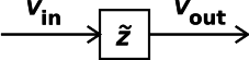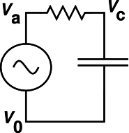
Figure 1: RC Circuit
Here are my notes on what a z transform is, and how it can be used to design and analyze digital filters.
As we shall see, it is often very convenient to express the real voltage V as the real part of a complex number V̂. Specifically:
| (1) |
where Re indicates the real part (of everything to its right). This V̂ is called a phasor, as described more fully below. Now Re is a linear operator, and multiplication by a scalar such as exp(iωt) is linear. That means they commute with any other linear operator. If you have a linear circuit and you want to calculate some function F (such as the input/output relation), then
| (2) |
which means that you can do the entire calculation in terms of the phasor V̂ and then find the actual voltage at the very last step, by multiplying by exp(iωt) and taking the real part.
It turns out to be very much simpler to keep track of a single complex number V̂ than to keep track of the amplitude and phase of the real voltage V, since amplitude and phase are nonlinearly related to the actual signal.
Be sure to heed the limitations and caveats in section 1.5 and section 1.6.
If the real voltage V has a sinusoidal waveform, it can always be written in the form:
| (3) |
for some real amplitude A, angular frequency ω, and phase φ0.
Equivalently we can write
| (4) |
where Re indicates the real part (of everything to the right), and CC stands for complex conjugate (of everything to the left). The sign convention is such that positive ω is what we call positive frequency. This sign convention is consistent with the more-or-less universal practice of writing the impedance of a capacitor as Z= 1/iωC, as discussed in connection with equation 11.
We can expand the exponential, so as to separate out the dependence on φ0:
| (5) |
So we have rederived the trigonmetric identity for the cosine of a sum. Note the minus sign on the last line. The fact is, if you choose zero phase to correspond to a cosine (not a sine) as in equation 3, and then you increase the phase by 90 degrees, you get a negative sine wave. This is an inescapable trigonometric fact.
This allows us to introduce the real-vector phasor representation:
| (6) |
where V1 and V2 can be considered the components of a two-dimensional vector. We call this vector the phasor representation of V. By comparison to equation 5, we can express the phasor components in terms of the amplitude and phase:
| (7) |
which can be inverted as:
| (8) |
The sign convention is such that when V1 and V2 are both positive, it corresponds to a positive frequency. The phasor (V1, V2) = (0, 1) is 90 degrees later than the phasor (1, 0).
Any vector in the two-dimensional plane can be represented as a complex number (and vice versa). For a phasor, that means:
|
where V̂ is a complex number, namely the complex phasor representation of V. We see that equation 9d is consistent with equation 6.
Note: If you think the minus sign in equation 6 seems ugly or inconvenient, rest assured that there has to be a minus sign somewhere, and the sign convention used here is (a) conventional and (b) vastly more convenient than any of the alternatives. We really want to have a plus sign in equation 9b, and we really want to have exp(iωt) to represent positive frequency. This pretty much requires a minus sign in equation 9d.
Note that when using the phasor representation, positive frequency corresponds to counterclockwise rotation in the plane (as it is usually drawn).
Let’s work a couple of simple examples, to show what phasors are good for.
Let’s consider differentiation with respect to time. Starting from equation 1, it is easy to show that
| (10) |
That is, differentiating the real voltage is equivalent to multiplying the phasor voltage by iω. This assumes that V̂ itself is constant, to a sufficient approximation. If V̂ is changing there will be additional terms on the RHS of equation 10, but if it is changing only slowly these terms will be small.
We can apply this to the AC current flowing in a capacitor.
| (11) |
where the last line can be seen as a generalization of Ohm’s law. This result can be summarized by saying the AC impedance of a capacitor is Z = 1/iωC.
By the same methods you can show that the AC impedance of an inductor is Z = iωL.
As an important application, you can find the input/output relation for the RC circuit shown in figure 1:
| (12) |
This is nothing more or less than the familiar voltage-divider formula, with the complex impedances plugged in. You see why this is called a low-pass filter. At low frequencies, it has a gain of 1. At high frequencies, the output is 90 degrees out of phase with the input, and when plotted on log-log axes, the gain falls off with a slope of 6 dB per octave, i.e. a factor of 2 in voltage for every factor of 2 in frequency, as shown by the dotted line in figure 5.
Now suppose we have a delay line that delays all signals uniformly, delaying them by a time τ, as indicated in figure 2
It is easy to show, starting from equation 1, that the voltage at the output is related to the voltage at the input by the simple relation:
| (13) |
where we define
| (14) |
Note that a factor of z makes the signal earlier, while z−1 makes the signal later. This famous “z transform” is named for this z. Note that the so-called z transform is not really a transform at all. It is just a collection of techniques that revolve around z and various powers of z, where z−1 is the phasor representation of a delay.
Let’s start with the familiar expression for Ohm’s law:
| (15) |
For linear AC circuits, we generalize this to
| (16) |
where Z represent the complex impedance. Let’s focus on the case where Z = R + 1/iωC for a resistor in series with a capacitor.
Another quantity of interest is the dissipated power:
| (17) |
The problem is, in the last two equations the symbol “V” is being used with two different, inconsistent meanings. We can clarify things by rewriting the two equations as:
| (18) |
| (19) |
The unadorned symbol V is ambiguous. It could be interpreted as V̂ or as V. Interestingly enough, equation 15 is equally valid under either interpretation. In contrast, the V in equation 16 must be interpreted as the phasor V̂ (as in equation 18, whereas the V in equation 17 must be interpreted as the real voltage V (as in equation 19). Because equation 17 is nonlinear, the phasor interpretation would be quite wrong. If you have a phasor, you simply must convert it to a real voltage before calculating the power. Otherwise you will get things spectacularly wrong.
For example, consider a wave with sine-like phase (as opposed to cosine-like phase). It is represented by a pure imaginary phasor. If you incautiously plug that into equation 17 and turn the crank, you will calculate a negative power, which is about as wrong as it possibly could be.
Notation that is convenient in one context is not always convenient in other contexts. Tradeoffs must be made. For example:
Suggestion: When you write, it is often helpful to include a legend or glossary, explaining what terminology you are using and what you mean by it. This applies to writing software as well as writing prose.
Example:
| (20) |
Some additional suggestions and caveats:
As for the term phase, sometimes it refers to the total phase
| (21) |
and sometimes it just refers to the initial phase φ0. I’m not going to argue that one is more correct than the other; they’re just different. To help reduce the ambiguity, it is a good habit to write a subscript 0 on φ0, and to use the word total when referring to the total phase.
As for the term frequency, if the frequency is constant then equation 21 is just fine. However, if the frequency is changing, for instance in the context of FM (frequency modulation), then we must consider the instantaneous frequency ω(t). The total phase becomes
| (22) |
Let’s be clear: If you naively write the phase as φ(t) = ωt + φ0 and then change the frequency, you will get wildly wrong answers.
As for the term amplitude, sometimes it refers to the A that appears in equation 3, in which case it could be positive or negative. Alternatively, sometimes amplitude refers to |A|. Another possibility is the RMS amplitude, which is about 30% smaller:
| (23) |
Sometimes instead of talking about the amplitude people talk about the peak-to-peak swing, i.e. 2|A|.
Quite often, people indicate what notion of amplitude they are using by putting subscripts on the units of measurement (rather than on the thing being measured). This is not the least bit logical, but it is so common that you might as well learn to tolerate it. Here are three equivalent ways of describing the same waveform:
| (24) |
The far more logical approach is to attach the “RMS” to the thing being measured (as in equation 23), rather than to the unit of measurement (as in equation 24). According to the SI system of units, there is no such thing as an “RMS” volt (Vrms) or a “peak-to-peak” volt (Vp-p) ... there is only the plain old volt (V).
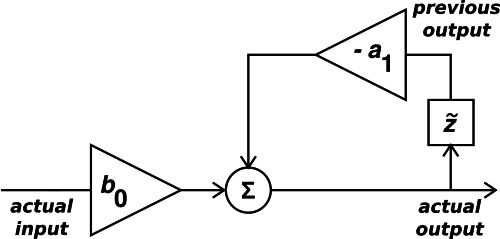
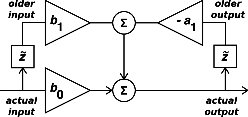
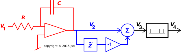
Let’s start with the simple example shown in figure 3. It involves a feedback loop, in which there is a delay line. (Basic delay-line concepts and terminology are discussed in section 1.4.)
From the point of view of digital filter design, this is not a high-performance filter, but it does have its uses. For one thing, it is often used in software to simulate an analog RC lowpass filter (figure 1). The feedback with delay allows the circuit to remember the previous output. The output gradually decays from the previous output value toward the current input value.
The diagram in figure 3 is equivalent to the following equation:
| (25) |
Commonly we set b0 equal to 1 − (−a1), so that the filter has gain=1 at frequency=0.
When the amount of feedback (i.e. −a1) is equal to 1, so that a1 = −1, the filter has infinite gain when ω=0, i.e. when z=1. At low frequencies (low compared to the Nyquist frequency), it behaves like a perfect integrator.
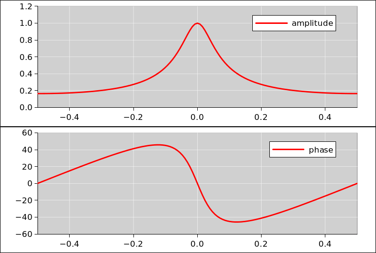
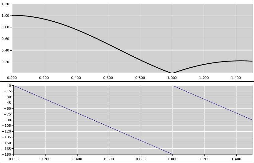
Note that all these expressions are implicitly a function of frequency, because z depends on frequency. We can evaluate the amplitude and phase of the transfer function (V̂out / V̂in as a function of frequency, directly from equation 25. The results are shown in figure 4.
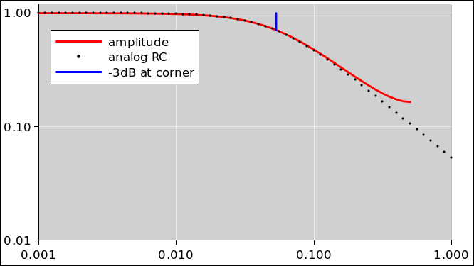
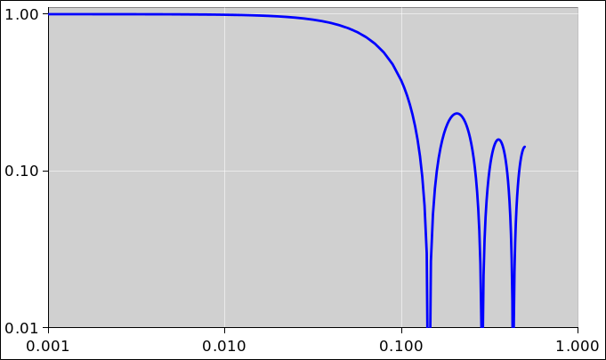
It is often instructive to look at the frequency response on log-log axes, as shown in figure 5. For comparison, this figure also shows the response of an analog RC lowpass filter (with the same corner frequency). We see that except at the highest frequencies (near the Nyquist frequency), the digital filter in figure 3 is quite a good model for the analog filter in figure 1.
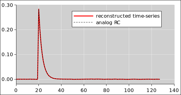
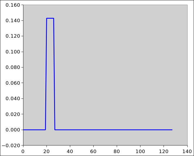
Last but not least, it is often worthwhile to look at the impulse response of the filter. This is shown in figure 6. You can see that the impulse response of the digital filter is remarkably close to the response of an old-school analog RC filter.
This is the response to a delta-function input at time t=20. The area under the curve is unity.
A generalization of this circuit is shown in figure 7. This will be discussed in section 2.9; see equation 41 in particular.
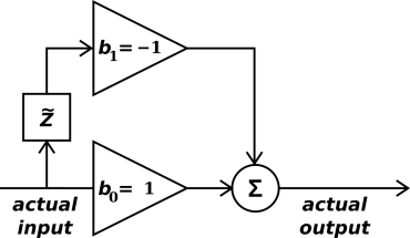
The circuit in figure 8 calculates the first differences. At low frequencies, it behaves as a perfect differentiator. More generally, it serves as a high-pass filter.
The equation is:
| (26) |
As usual, we assume b0=1.
So when b1 = −1, there is a zero at DC (where ω=0 and z=1) and a pole in the middle of the z-plane (where z=0). At low frequencies, this behaves as a perfect differentiator.
This is an example of a filter with Finite Impulse Response (FIR). There is no feedback, so after a few samples it has completely forgotten any history it had.
If we take the previous circuit and change b1 to +1 we get:
| (27) |
which has a zero at z=−1, i.e. when the frequency is equal to half the sampling frequency.
If instead we add a second delay element, so that b1=0 and b2=−1, we get:
| (28) |
which has zeros at both z=1 and z=−1. It clobbers DC and it also clobbers the Nyquist frequency.
Suppose we want a zero on the |z|=1 unit circle at some frequency f. Necessarily there will be another zero at negative frequency.
| (29) |
which tells us the coefficients to use for the taps in our filter.
Almost anything you want to do with a FIR (zeros-only) filter can be done by stacking stages of the form given by equation 29. The only exceptions have already been covered, in equation 26, equation 27 and equation 28.
You can stack stages explicitly, by feeding the output of one simple filter into another simple filter ... or you can implement the whole stack in a single multi-tap filter. Multiply the polynomials to find the coefficients.
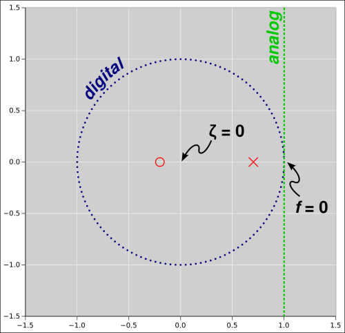
Let’s write an equation with the same general form as equation 25, except as a function of some arbitrary complex number ζ (Greek letter zeta) ... instead of z. We let ζ vary over the entire complex plane ... in contrast to z, which is confined to the unit circle, since it is defined as z = exp(iωτ). Beware that people commonly gloss over the distinction between ζ and z, and speak of «the complex z plane» but that’s not entirely logical.
| (30) |
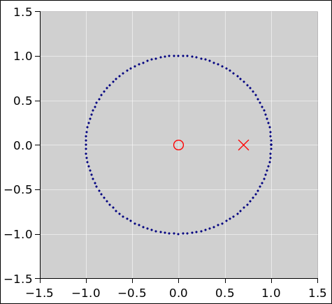
It could be argued that the only thing that actually matters for calculating the filter response function is the special case where we set ζ = z ... but we are allowed to at least imagine other values of ζ, and plot other values of ζ. Such a plot gives us a nice overview of the situation, as shown in figure 9.
The figure represents the complex plane as a whole. The variable ζ can be anywhere in the complex plane. The circle represents the important special case where ζ = z. On the circle, the 3:00 position corresponds to zero frequency (z=1). The 12:00 position corresponds to half of the Nyquist frequency (z=i). The 9:00 position corresponds to the full Nyquist frequency (z=−1). The lower half of the circle corresponds to negative frequencies.
In addition, we note that equation 30 has a pole at ζ = −a1 and a zero at ζ = 0. These locations are plotted in the figure. Because the functional form of the transfer function is an analytic function, indeed a rational function, thinking in terms of poles and zeros gives us tremendous insight into what the filter is doing. The transfer function can be visualized, roughly, as a membrane that is pushed up by the poles and pinned down by the zeros. When z is near a pole, the transfer function will be large ... and when it is near a zero, the transfer function will be small.
When the signal frequency is f=0, we have z=1. This follows directly from the definition of z in equation 14. The situation is shown in figure 10.
This creates opportunities for confusion and miscommunication. For example, if somebody says there is a «pole at zero» you might have no idea whether that means f=0 or ζ=0.
Also in figure 10, you can see the relationship between analog filter design and digital filter design. For low enough frequencies – near f=0 – the difference is unimportant; a digital filter can do anything an analog filter can do. However, an analog filter can get arbitrarily far away from f=0, whereas a digital filter cannot. A digital filter is stuck on the |ζ|=1 circle.
Note that the direction of real frequency is vertical in this diagram ... whereas the real part of ζ is horizontal. This is another source of confusion and miscommunication. For example, if somebody says such-and-such feature is located on the real axis, you might have no idea what that means.
Here’s another important concept: In the figure there is a pole three tenths of a unit away from f=0. This does not, however mean the pole is at f=0.3 or anywhere close to that. Instead, the pole is 0.3 units away in the direction perpendicular to the f-axis, if we are thinking in analog terms. In digital terms, we can say something similar: The pole is 0.3 units away from the |ζ|=1 circle.
By the same token, in the figure there is a zero two tenths of a unit away from ζ=0. It is nowhere near f=0.
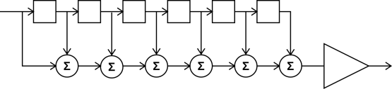
A boxcar average is another not-very-high-performance digital filter. We are not recommending it.
| Nevertheless, it is rather commonly used. For one thing, it is extremely simple to compute ... and if you do it cleverly, a large-N boxcar requires no more additions or multiplications than a small-N boxcar. Also, the boxcar average is relatively easy to understand. If the input is a sine wave at a frequency such that an integer number of cycles fit evenly into the boxcar, the output is zero. Another reason for paying attention to this circuit is that it is easy to analyze, using the same techniques as in section 2.1. It is a good exercise, to build up experience and confidence in z-transform methods. | Disadvantages include the following: If you are using it as a notch filter, it is not very convenient, because the zeros are not easily moveable; they are stuck at integer submultiples of the sampling frequency. Also, the filter response is not very flat within the passband. You can obtain much better performance by moving those poles away from the origin. This is easy to do using biquads, as discussed in section 2.9. |
Remark: Terminology: We have to watch out for a fencepost issue: Here N is the number of points. An N-point moving average requires N taps but only N−1 delay boxes, because you get the zeroth one for free. In figure 11, the taps are labeled 0 through 6 inclusive, for a total of N=7.
The transfer function is:
|
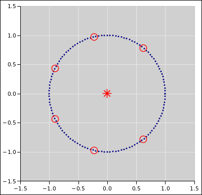
Again we generalize this from a function of z to a function of ζ. The numerator of equation 31b tells us there must be six zeros, although it is not yet obvious where. The denominator tells us there are six poles (all at ζ=0).
The next step is to use equation 31c, which makes it easy to see where the zeros are. At first glance it might look like there could be a zero at z=1, but the would-be zero is canceled by a pole at z=1.
Let’s be clear: The appearance of a 7th power in equation 31c does not mean there are 7 poles or zeros. There is a factor of (1−z) in both the numerator and denominator, which cancel, so in actuality there is neither a pole nor a zero at z=1. This shared factor was introduced when we went from from equation 31b to equation 31c. The reasoning goes like this: The six actual zeros are all the 7th roots of unity, excluding the one at z=1.
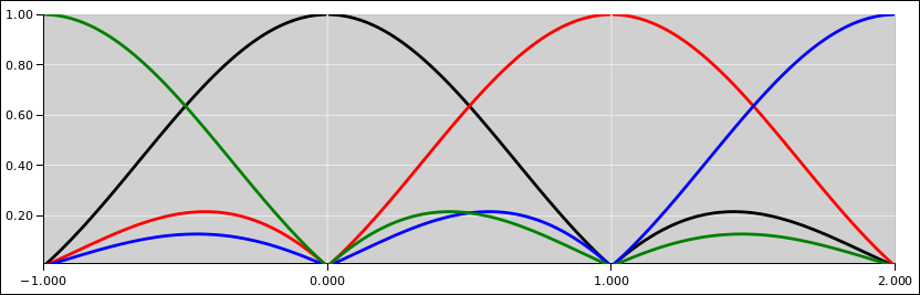
The pole-zero plot is shown in figure 12. The general rule an N-point boxcar is that there will be N−1 zeros and N poles, where N=7 in our example. All the poles are on top of each other at ζ=0. The zeros are located at N−1 of the Nth roots of unity. That is to say, raising the z-location of each root to the N power gives unity.
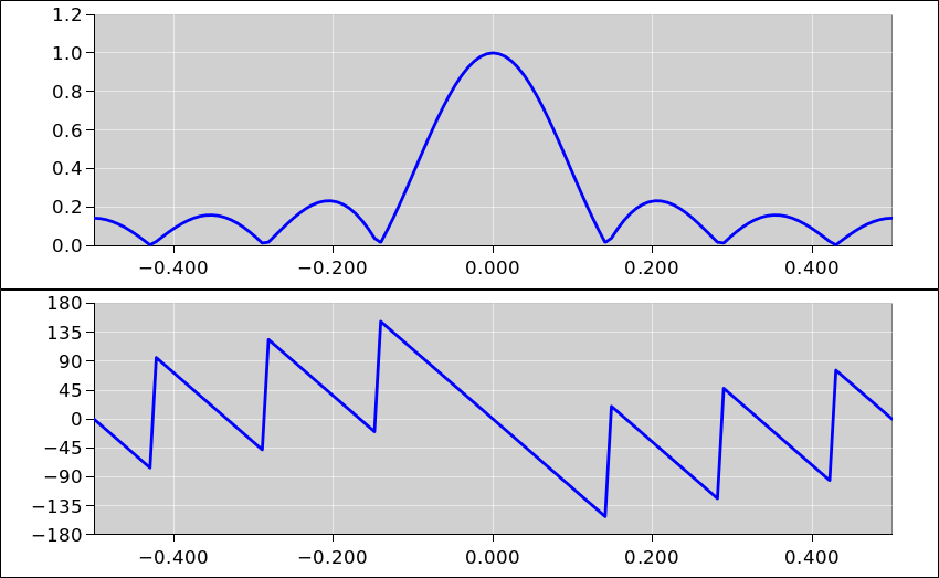
Here is the plot of phase and amplitude.
Here is the amplitude on log/log axes.
Here is the impulse response.
Almost any A-to-D system involves sampling the waveform at discrete times. We idealize this in terms of a zero-width sampling window that repeats at intervals of Δt. That is to say, the sampling function is modeled as succession of delta functions, i.e. a Dirac comb. This can also be called the stroboscopic approach. That’s fine as far as it goes, but it cannot possibly be the whole story.
To see what’s involved in measuring a signal, let’s do an example. Although this example seems logical, it will turn out to be somewhat less than satisfactory. In any case it serves as a useful warm-up exercise. We proceed as follows: For every measurement interval, measure the average of the signal during that interval.
As usual, the average over time of X is defined as
| (32) |
The denominator is just Δt. The numerator can be expressed in the usual way as the difference between two indefinite integrals.
| (33) |
To a first approximation, one way to implement this starts with the circuit sketched in figure 16. There is an analog integrator (shown in red) followed by a differencer (shown in blue), followed by sampling at discrete intervals (shown in black). For pedagogical reasons, we imagine that the differencer is implemented using an analog delay line. This is certainly possible, although in practice it would make more sense to move the sampling upstream of the differencer, and do the delay in software. Still, though, analog delay lines do exist, so this is not completely crazy. Since it is a linear system, the operations can be performed in any order, and the answer comes out the same.
The analog filter has a pole at f=0. The differencer has a zero at f=0 and a pole at ζ=0. We can calculate that as follows: Using basic principles such as the definition of capacitance, we find that
| (34) |
where the unity-gain frequency is
| (35) |
For the differencer, we can immediately write
| (36) |
This formula applies equally well to analog differencer implementations and to the corresponding digital implementations.
In any case, the transfer function of the integrator and differencer together is the product of two factors:
| (37) |
Unlike a filter based solely on delay elements, this cannot be expressed as a rational function of z, because of the first factor. On the other side of the same coin, the second factor cannot be expressed in terms of any finite number of resistors and capacitors.
Keep in mind that z=1 and f=0 mean the same thing, so at sufficiently low frequencies, the numerator in the second term cancels the denominator in the first term. The combination of integrator and differencer together exhibits neither a pole nor a zero near f=0. We can understand this in more detail if we expand z as follows:
| (38) |
Note that θ is measured in radians, while almost everything else is measured in cycles. In particular f is measured in Hz. This θ is the angle as seen from the center of the |ζ|=1 circle. At the Nyquist frequency, θ=π and z=−1.
Then we can expand the transfer function as
| (39) |
The phase and magnitude of this transfer function are shown in figure 17. We have scaled the vertical direction so that the magnitude is unity at DC, and we have scaled the horizontal direction so that 1/Δt corresponds to unit frequency.
Discussion: Note that the function (exp(α)−1)/α is sometimes called expc(α). See reference 1 and reference 2. For pure imaginary α=iθ, its imaginary part is the relatively familiar sinc(θ) function, but the full expc function is even more interesting. It does not even remotely resemble a Dirac comb. If you zoom out on an expc function, rescaling the height and width, it eventually resembles a single delta function, never a Dirac comb. This shows that the stroboscopically sampling the signal at regular intervals is never going to be the whole story. Some sort of analog filter is absolutely needed upstream of the digitizer.
There is a way of understanding the linearity of the phase as a function of frequency. For any given point on the |ζ|=1 circle the angle θ, i.e. the angle as seen from ζ=0. Also consider the angle β, which is the angle as seen from ζ=1, which is also the phase of (z−1). You can draw an isosceles triangle and convince yourself that as θ goes from zero to 2π, β goes from zero to π.
These two parts of the circuit are still analog circuits. They can process signals well above the frequency set by the Δt in the analog delay line.
This example shows that the formulas involving z apply even to analog delay lines. Such formulas can be combined with formulas from the analog world, even if the overall result cannot (so far as I know) be diagrammed in terms of poles and zeros on the complex ζ plane or on the complex s plane, or any other plane that I know of.
The module shown in figure 16 is not practical by itself. For one thing, a DC input would cause the integrator to integrate to infinity. There are lots of ways of fixing this problem, for instance by making the module part of a larger system, within a feedback loop.
We now consider the effect of sampling the signal. Multiplication in the time domain is equivalent to convolution in the frequency domain. Remarkably enough, the Fourier transform of a Dirac comb is a Dirac comb. So we have to convolve the curves in figure 17 with a Dirac comb. Figure 18 shows the first four contributions.
Let’s focus attention on the interval between 0 and 1. In this interval, all four terms contribute. Keep in mind that this is just four terms of an infinite series. The series doesn’t even converge, so we have quite a mess on our hands. We conclude that a simple integrator doesn’t get the job done. We need at least a two pole low-pass filter in front of the sampling stage; otherwise the signal will get massacred by all the aliasing.
A biquadratic filter produces two poles and two zeros. It can easily be configured to put the poles and zeros anywhere you want. If you want more than two poles and zeros, standard engineering practice is to use multiple biquads, i.e. multiple stages in series ... rather than building more complicated filters with a more poles and zeros per stage.
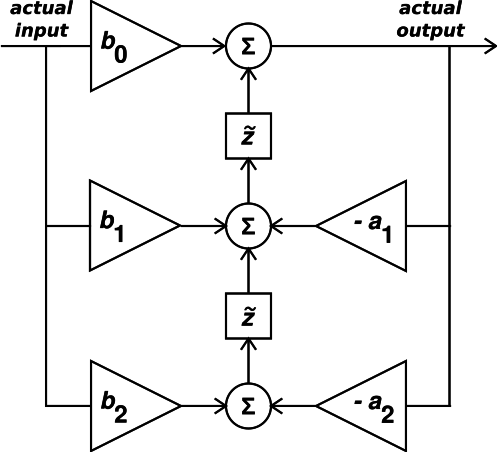
There are about a dozen ways of implementing a biquad, all of which produce the same results. The arrangement in figure 19 is called “Direct Form II Transposed” and is simple to implement in C++ code, and also simple to analyze.
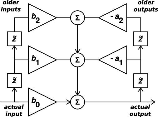
Meanwhile, the arrangement in figure 20 is called “Direct Form I”. It may appear unnecessarily complicated, insofar as it require four delay registers (whereas figure 19 only requires 2). However, if you are implementing this on a spreadsheet, where you have the older inputs and older outputs lying around anyway, this form is quite convenient. It is just as easy to analyze.
Here’s the analysis for Direct Form II:
|
In equation 40d we re-expressed the result in terms of z rather than z̃, which is a more conventional and more convenient form. However, this means that in the numerator, c0 is the coefficient in front of z2 while c2 is the coefficient in front of z0, which is kinda backwards and is a trap for the unwary.
The big advantage of equation 40d is that the poles and zeros of V̂out/V̂in correspond to the high points and low points of the filter response function. Loosely speaking, we get to re-use some intuition that we have about analog filter design, which also involves poles and zeros.
From the structure of equation 40d it is clear that this circuit can implement any input/output relation that has at most two zeros and at most two poles. All we have to do now is choose the coefficients appropriately.
In the special case where the coefficiences b2 and a2 are both zero, the biquadratic filter becomes merely a bilinear filter:
| (41) |
which has a pole at z=−a1 and a zero at z=−b1/b0. An example in this category is the simple low-pass discussed in section 2.1.
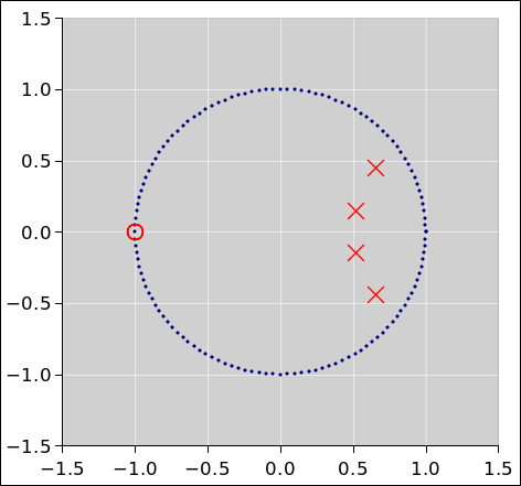
Let’s assume – temporarily – that our two poles are a complex-conjugate pair. Poles are not always of this form, but often they are. So, one pole is at z0 = x + iy and the other is at z0 = x + iy, for some given real numbers x and y. We can calculate the filter coefficients as follows. Poles of the transfer function are zeros of the denominator, i.e. the following polynomial:
| (42) |
and from that we can read off the coefficients:
| (43) |
or in (r, θ) polar coordinates:
| (44) |
We now lift the assumption that the poles are a complex-conjugate pair. If the poles are on the real axis, they don’t have to be paired. Then we are looking for solutions to the equation (z−p)(z−q) for some given real numbers p and q.
| (45) |
There is no advantage to writing things in polar coordinates in this case.
Some remarks about the real axis:
Let’s look again at figure 19 and the corresponding equation 40d. The b coefficiencs have to do with delayed copies of the input, and they wind up in the numerator. The a coefficients have to do with delayed copies of the output, and they wind up in the denominator.
If all the a coefficients are zero, we have a FIR filter, i.e. finite impulse response. There is no feedback; it’s all feed-forward. One might say that in the z̃ plane such a filter has zeros but no poles ... but more to the point, in the z plane it has a bunch of zeros, each of which is paired with a pole at the z=0. The boxcar average is in this category.
All the other filters discussed in this document are IIR i.e. infinite impulse response. Almost any circuit with nontrivial feedback will be in this category. As a matter of principle, the impulse response goes on forever, but if all the poles are inside (not on) the unit circle in the complex ζ plane, the impulse response will be exponentially small at long times.
Suppose you would like to build an N-pole Butterworth filter. This is known to have good properties such as minimal ripple in the passband. Some free, open-source, GPL software for figuring out the placement of the poles and zeros is available via reference 3.
The design for a four-pole Butterworth low-pass filter are shown in figure 21. There is a little archipelago of poles. If we extrapolate the archipelago, it intersects the z-circle at the corner frequency of the filter.
There is is a quadruple zero at z=−1.
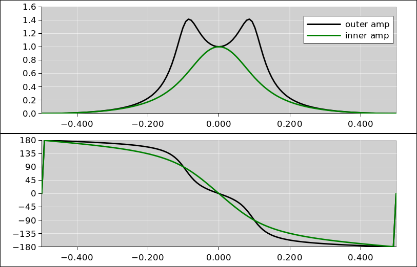
Looking at figure 21 we see two pairs of poles. We implement these using stages, i.e. two biquads in series: one for the “innner” pair and one for the “outer” pair. The amplitude and phase of the two transfer functions are shown in figure 22.
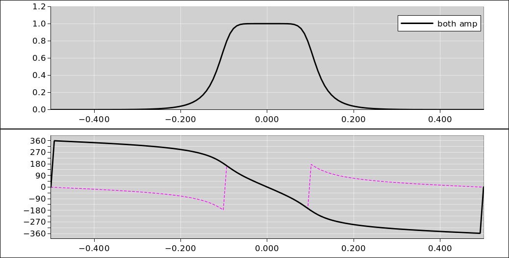
When we multiply the two stages together, we get the overall transfer function shown in figure 23.
In this figure, the “conventional” phase is shown with a dashed magenta curve. This is the conventional branch of the arctangent function, and is confined to the region from −180 to +180 degrees of phase. Alas, this is phenomenally ugly, since there is a branch cut right near the corner frequency of the filter. The black curve presents exactly the same phase information, but splices together three different branches, to make it clear that there is no discontinuity.
Contrast this with the boxcar as shown in figure 13, where the phase really is quite discontinuous, and you can’t fix it by adding or subtracting 360 degrees. The phase changes by 180 degrees every time z goes past one of the zeros.
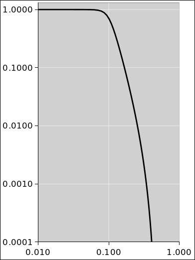
It is nice to look at the amplitude on log/log axes, as we see in figure 24.
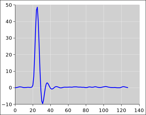
The impulse response is shown in figure 25. Note that it exhibits some ringing. This is the price that must be paid for having a passband with steep sides. If you cannot tolerate ringing, use a filter with lower Q. A boxcar average obviously cannot ring. Also a Gaussian filter cannot ring; the Fourier transform of a Gaussian is a Gaussian.