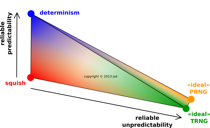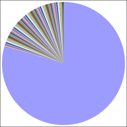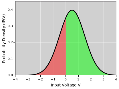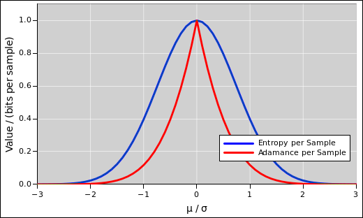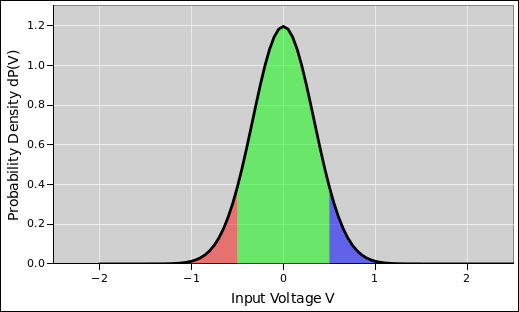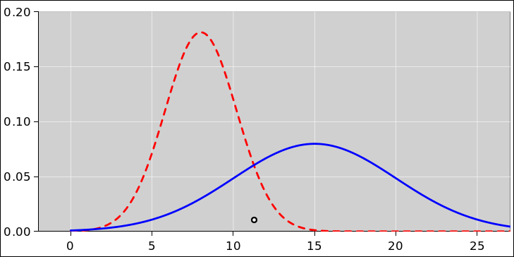
Figure 1: One Point, Two Distributions
ABSTRACT: We discuss how to design a so-called Random Number Generator (RNG). More precisely, we are interested in producing a random distribution of symbols (numerical or otherwise). Such distributions are needed for a wide range of applications, including high-stakes adversarial applications such as cryptography and gaming. You can do a lot better using physics and algorithms together than you could with either one separately.
A fundamental building-block is a so-called Hardware Random Number Generator (HRNG), which closely approximates an ideal True Random Number Generator (TRNG). It starts with a raw signal derived from some fluctuating physical system. It then processes that signal to remove biases and correlations. The hash saturation principle – basically a pigeonhole argument – can be used to prove that the output has the desired statistical properties.
It is essential that the underlying physical system be calibrated. We require a strict lower bound on the amount of thermodynamic unpredictability, not merely an estimate or an upper bound. The lower bound must come from the laws of physics, since statistical tests provide only an upper bound. The details of the calibration process will vary from system to system. A remarkably cost-effective example uses standard audio I/O hardware, as discussed in reference 1.
The output of the HRNG can be used directly, or can be used to seed a so-called Pseudo Random Number Generator (PRNG).
róbungy
There is a wide range of important applications that depend on being able to draw samples from a random distribution. See section 2.3 for an overview of some typical applications. Some of the things that can go wrong are discussed in section 6.1.
Here is one way to construct a so-called Hardware Random Number Generator (HRNG). We want it to closely approximate an ideal True Random Number Generator (TRNG) – suitable for a wide range of applications, including extremely demanding ones.
We start by introducing some key theoretical ideas:
It must be emphasized that there is no such thing as a random number.
Figure 1 illustrates this idea. Consider the point at the center of the small black circle. The point itself has no uncertainty, no width, no error bars, and no entropy. The point could have been drawn from the red distribution or the blue distribution. You have no way of knowing. The red distribution has some width and some entropy. The blue distribution has some other width and entropy.
Terminology: Therefore a so-called «random number generator» (RNG) must not be thought of as a generator of random numbers; rather, it is a random generator of numbers. Furthermore, it often useful to generate a random distribution over non-numerical symbols, in which case the term RNG should be interpreted to mean randomness generator or something like that.
Terminology: If you ask three different people, you might get six or seven different definitions of “random”.
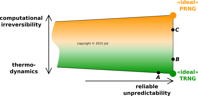
At a minimum, we need to consider the following ideas, which are diagrammed in figure 2.
For example: Once upon a time I was working on a project that required a random distribution. The pointy-haired boss directed me to use the saved program counter at each interrupt. I had to explain to him that it was an event-driven system, and therefore the saved PC was almost always a constant, namely the address of the null job. Of course it was not reliably a constant, but it was also not reliably unpredictable. There was no positive lower bound on the amount of randomness. In other words, it was squish.
The terminology is not well settled. I have heard intelligent experts call items 1, 2, 4, and 5 on the previous list “random”. I have also heard them call items 3, 4, and 5 “non-random” or “not really random”. Sometimes even item 2 is included in the catagory of “not really random”.
Additional remarks:
As you can see in figure 2, there is a continuum of possibilities along the line from ideal TRNG to PRNG ... and a lot of other possibilities besides.
Figure 3 is a close-up, top-down view of the rightmost part of figure 2.
Let’s discuss the three labeled points: A, B and C.
Such things can be made good enough for some purposes. The house take for an ideal roulette wheel is a few percent. From the house’s point of view, if the wheel is skewed by more than that, it is a disaster for the house, as discussed in reference 2. In contrast, a small amount of skew (perhaps a few parts per million) is not worth fixing. Indeed the house will sometimes intentionally give away a percent or two for marketing purposes; In Las Vegas, for example, high-stakes players may be offered a single-zero wheel, or offered partage. From the player’s point of view, a tiny skew in the wheel statistics is not worth exploiting; it would cost a fortune to measure the statistics sufficiently carefully, and would detract from whatever entertainment value the game offers.
Alas, a device that is good enough for gambling may not be good enough for cryptography. Imagine using a roulette wheel to directly generate one-time pads. If you send a large number of messages with such a system, it is possible that your adversary may be able to exploit the statistical flaws.
You could try to make a better hardware-only RNG, moving rightward from point A in the diagram ... but in many cases it is cheaper and better to move diagonally, from point A to point B.
In practice point B differs from point C by an enormous amount, far more than is suggested by the diagram. Point B may rely on algorithms for only 10−5 of its randomness, while point C may rely on physics for only 10−9 of its randomness ... so in this scenario the two RNGs differ by 14 orders of magnitude. That’s not infinite, but it’s a lot. It may be enough to cause the attacker to choose a different line of attack in the two cases.
It must be emphasized that an «ideal» PRNG cannot possibly exist. Any real PRNG depends on an internal state that must be initialized; that is, the PRNG needs a seed. That leaves us with a question: where does the seed come from? If it comes from another PRNG, it reduces to the problem previous not solved: Where did the upstream PRNG get its seed? The only way to avoid infinite regress is to use physics, to use a hardware RNG to provide the seed.
“Anyone who considers arithmetical methods of producing random digits is, of course, in a state of sin. For, as has been pointed out several times, there is no such thing as a random number – there are only methods to produce random numbers, and a strict arithmetic procedure of course is not such a method.” – John von Neumann (reference 3)
Let’s be clear about the contrast:
| It is possible to have a RNG that relies completely on physics without needing any cryptologically-strong algorithms. Example: Roulette wheel. | It is absolutely not possible to have a RNG that relies completely on algorithms without needing any physical source of randomness. The seed has to come from somewhere. |
However, it would be difficult if not impossible to build a hardware-only RNG that is good enough for the most demanding applications. You can get more strength, higher data rates, and lower cost by using a hybrid approach, using both thermodynamics and cryptography.
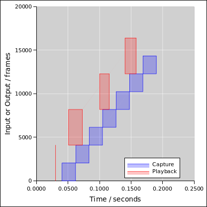
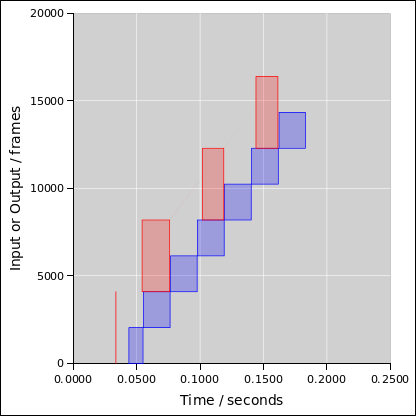
This sometimes limits the usefulness of the HRNG. This can be very significant, because on many systems the peak demand for randomly-distributed symbols is very spiky. That is, the peak demand is many orders of magnitude greater than the average demand.
One seemingly-obvious way of dealing with the spiky demend is to buffer the output of the HRNG. However, this undercuts one of the main selling points of the HRNG, since the buffer constitutes a stored state that the adversary can capture. So once again we find that the difference between a practical HRNG and PRNG is a matter of degree, not a categorical difference.
If the RNG is being used for a cryptographic application, you can presumably always use the same crypto primitives in the RNG that you use in the application. Then you don’t need to worry too much about cryptologic attacks on the RNG, because anything that breaks the RNG will also break the application directly, even worse than it breaks the RNG.
To be clear: There are standard techniques for using a block cipher to create a cryptologically-strong hash function. This is one way of providing the one-way property that the RNG requires.
There exist a number of “old-school” hardware-only methods for generating random distributions. This includes
Such methods are supposed to derive their randomness directly from physics, without computing any cryptographically-strong algorithms – indeed without using any computer at all.
A “powerball” machine is supposed to be tamper resistant, but in practice the tamper-resistance is far from perfect; see reference 6. A skilled cardsharp can perform a controlled shuffle that is not random at all; see reference 7. Similarly there is a controlled coin toss; see reference 8
Even when the hardware has not been subjected to tampering, it might not be random enough for the purpose; see reference 8 and reference 2.
Given a distribution P, the ith possible outcome is observed with probability Pi.
We define the surprisal aka surprise value of the ith possible outcome to be:
| $i := log(1/Pi) (1) |
Given a distribution, there are lots of things we might want to know about it. There is not any one “best” tool for characterizing a distribution. The available tools can be used in combination, and the details depend on what we’re trying to accomplish.
For any distribution P, the available tools include the family of Rényi functionals, denoted Hα[P], where α is called the order of the Rényi functional. The meaning is particularly clear for three special values of α:
|
where the sums and the Min operations run over all symbols that can be drawn from the distribution with nonzero probability.
The formal, fully-general definition of the Rényi functionals is given in section 1.9.
Remarks:
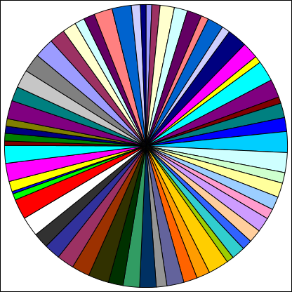
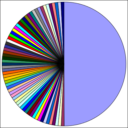
Some example distributions are shown in figure 4 and figure 5.
| The distribution in figure 5 has the following properties: | The distribution in figure 6 has the following properties: |
The relatively simple distributions in figure 5 and figure 6 can be generalized in various ways, including the following: Suppose there are N codes. One of them has probability q, and the remaining codes evenly share the remaining probability, so that they have probability (1−q)/(N−1) apiece. It is then easy to show that the distribution has the following properties:
|
The following table shows some illustrative values. We consider the case where the symbols are 256-bit words, so N = 2256. We examine various values of q, and plug into equation 6.
| q | H0 | S | H∞ | |||
| 0.5 | 256 | 129.0000 | 1.0 | |||
| 10−3 | 256 | 255.7554 | 10.0 | |||
| 10−6 | 256 | 255.9998 | 19.9 |
This shows that the plain old entropy really doesn’t tell you everything you need to know. In the last line in the table, the entropy is very nearly as large as it possibly could be, yet the outcome is predictable one time out of a million. That’s about 70 orders of magnitude more predictable than it would be if the distribution were truly random.
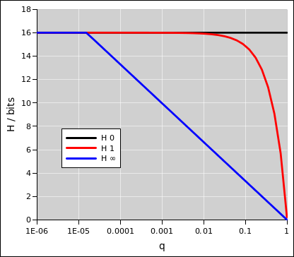
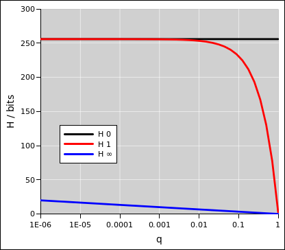
The same idea is illustrated in figure 7 (for a 16 bit word) and figure 8 (for a 256 bit word). Knowing that the entropy is very high is not sufficient to guarantee that the outcome is unpredictable.
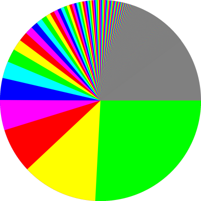
An even more extreme example is shown in figure 9. The distribution has infinite entropy. This is arranged using techniques described in reference 9.
In more detail, the distribution in figure 9 has the following properties:
This serves as one more warning that the entropy is not always a good measure of resistance to guessing.
The entire family of Rényi functionals can be defined as follows, for any order from α=0 to α=∞:
| (8) |
Again, the sum runs over all symbols that can be drawn from the distribution with nonzero probability. Note: In the important special case α=1, you can use l’Hôpital’s rule to get from equation 8 to equation 2b.
It is easy to prove the following inequalities:
| (9) |
That means that when H∞ approaches its maximum possible value, the entropy is also large, and all three measures are very nearly equal. However, the reverse is not true. When the entropy is large, even when it is very nearly equal to H0, the H∞ value might be quite low ... as we see in table 1.
It is also easy to prove that the Rényi functional (of any given order) is additive when we combine independent probabilities. That is:
| (10) |
for any α, provided the distributions Q and R are statistically independent, where
| (11) |
By definition, “independent” that means the probabilities are multiplicative:
| (12) |
for all i and j. It is easy to prove that if the probabilites are multiplicative the Rényi functional is additive, using little more than the definition (equation 8) plus the distributive law.
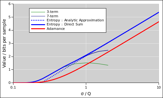
We shall make heavy use of this result. In particular, for a string of symbols, where successive symbols are independent and identically distributed (IID), the entropy of the string grows in proportion to the length of the string, and the adamance also grows in proportion to the length of the string.
The adamance H∞[P] is a minimax measure of the guessability, since it measures how hard it is to guess the most easily guessible symbol that could be drawn from the distribution.
| (Since H∞[P] is a minimax measure, calling it the «min-entropy» would be a misnomer of the kind that leads to misconceptions. There are lots of other concepts that have at least as good a claim to represent some kind of “min” entropy.) |
To say the same thing another way:
To appreciate the distinction between entropy and adamance, refer again to figure 9. It has infinite entropy but finite adamance. In some sense virtually all of the codewords are infinitely hard to guess, but the most-guessable codewords are not very hard at all.
In figure 9, the adamance is limited by the large “soft spots” i.e. low-surprisal codewords. You can increase the adamance somewhat by deleting the most-probable codewords and renormalizing what’s left, but the results are disappointing. You can delete any finite set of codewords and the distribution will still have infinite entropy and finite adamance.
The concept of entropy as used in classical cryptology and information theory is exactly the same thing as the concept of entropy as used in classical physics. In other words, the Shannon entropy is exactly the same thing as the Boltzmann entropy. Checking the equivalence is simple in some cases and complicated in others, but it has been checked.
In the unlikely event that you are dealing with entangled Schrödinger cat states, a fancier definition of entropy is required ... same idea, more general formula. Even then, the cryptological entropy remains the same as the physics entropy. Unsurprisingly, you need to upgrade both sides of the equivalence.
In all cases, entropy is defined in terms of probability. You can dream up lots of different probability distributions. If you use an unphysical distribution, you will get an unphysical value for the entropy.
Entropy is the answer to some interesting and important questions. It is not, however, the answer to all the world’s questions.
Adamance and entropy are defined in terms of probability. In the same way, we can define conditional adamance and conditional entropy, defining them in terms of conditional probability. The same idea applies to other types of random distributions, including pseudo-random distributions. For more on this, see section 6.4.
As discussed in section 1.2, there is a world of difference between a distribution and a symbol that may have been drawn from such a distribtion.
The surprisal is by definition a property of the symbol. In contrast, the multiplicity, entropy, and adamance are properties of the distribution.
The only way to define entropy or adamance for a single symbol is to define a new distribution containing only that symbol, in which case the entropy and the adamance are both zero. In physical terms: if you thoroughly shuffle a deck in the usual way, the entropy and the adamance are both log(52!). However, if you shuffle it and look at the result afterward, then the adamance and the entropy are both zero.
In this section, we give a broad outline of what is possible and what is not possible; a more detailed discussion of objectives and tradeoffs can be found in section 2.2.
The basic objective is to provide a random distribution of symbols, with quality and quantity suitable for a wide range of applications.
In the interest of clarity, let’s consider a specific use case and a couple of specific threat models. (Some additional applications are listed in section 2.3. Some additional attacks are discussed in section 6.1 and section 6.3.)
Imagine that we are sending encrypted messages. The RNG is used to create an initialization vector for each message. There are two cases to consider:
Here are some of the criteria on which a random generator can be judged:
In particular, hypothetically, an encrypted counter would make a fine PRNG if we disregarded the anti-backtracking requirement.
This is a tricky requirement. In some sense rapid recovery is desirable, but it is not the main requirement, and there are limits to what can be accomplished. It’s like a seatbelt in an airliner. It protects you against injury during routine turbulence, but if the aircraft explodes in midair the seatbelt is not going to do you a bit of good. Spending precious resources on «better» seatbelts would make the overall system less safe. The point is, the primary defense against compromise is to design the overall system so that compromises are extraordinarily rare.
Secondarily, it may be that cryptanalysis allows the attacker to ascertain one or two bits of the internal state. The RNG should make it computationally infeasible for the attacker to exploit this information, and the RNG should be re-seeded often enough to ensure that this information is lost before it accumulates to any significant level.
Let’s be clear: Constanty re-seeding the PRNG is a bad idea. It wastes CPU cycles, and more importantly it wastes the randomness that is being taken from the upstream HRNG that is providing the seed material. If you are constantly worried about compromise, the solution is not more re-seeding; the solution is to redesign the system to make it more resistant to compromise.
In particular, if an attacker can cause the PRNG to re-seed itself frequently, it becomes a denial-of-service attack against the upstream HRNG.
These criteria conflict in complex ways:
These conflicts and tradeoffs leave us with more questions than answers. There are as-yet unanswered questions about the threat model, the cost of CPU cycles, the cost of obtaining raw entropy, et cetera. The answers will vary wildly from machine to machine.
Here is a list of typical applications where some degree of randomness is needed, followed by a discussion of the demands such applications place on the random generator:
The first three items require a random distribution with good statistical uniformity and independence, but do not usually require resistance against cryptanalytic attack. The molecules in a Monte Carlo simulation are not going to attack the Random Generator. Similarly, the shuffle used in a low-stakes game of Crazy Eights does not require a cryptographically strong RNG, since nobody is going to bother attacking it.
As the stakes get higher, the demands on the RNG get stricter. Implementing a multi-million dollar lottery requires the RNG to have excellent tamper-resistance as well as good statistical properties.
Game players need randomness, too. In the simple scissors/paper/stone game, choosing a move at random is the minimax strategy. More sophisticated games like poker require a mixed strategy, i.e. a mixture of deterministic and non-deterministic considerations. You must study the cards, study the other players, and sometimes make an unpredictable decision about whether to bluff or not.
Cryptography is far and away the predominant high-volume consumer of high-grade entropy. This is what motivated our search for better generators. Even a smallish secure-communications gateway can draw millions of bits from the random distribution in a one-minute period.
Item #7 requires special comment: Suppose you need to initialize the internal state in a PRNG. As discussed in section 1.3, at some point this requires a HRNG.
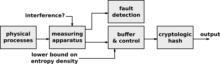
Figure 10 shows a block diagram of a High-Quality Random Generator. The symbols it generates are very nearly as random as possible.
The starting point for an HRNG is the unpredicability associated with one or more physical processes, such as radioactive decay or thermal noise. Such physical processes are partially random, in the sense that they contain contributions which are believed to be extraordinarily difficult for anyone to predict, perturb, or replay.
The raw symbols (as sampled from the data-acquisition apparatus) will, in general, be partly predictable and partly unpredictable, as discussed in section 6.4. The raw symbols are essentially 100% resistant to the attacks that plague PRNGs . That’s because those attacks are directed toward capturing the internal state, and the HRNG doesn’t have any internal state worth capturing.
Let’s consider an example. As always, the raw data comes from a physical process that produces some randomness. For simplicity, let’s toss a bent coin. It comes up heads 90% of the time and tails 10% of the time.
We consider one toss to be one symbol. We can encode such a symbol using one bit, or using 7-bit ASCII, or using an 8-bit byte, or using a 32-bit word, or whatever. It doesn’t matter, because the multiplicity is 2 possibilities per symbol. In more detail:
| (13) |
Next, consider a string consisting of three symbols from the same source. There will be 8 possible strings. We assume the symbols are independent and identically distributed (IID). We can characterize the statistics of the strings as follows:
| (14) |
Similarly for a string of seven symbols, there will be 128 possible strings. In more detail:
| (15) |
Even finer details of the calculation are shown in the following table:
| # of tails (k): | 0 | 1 | 2 | 3 | 4 | 5 | 6 | 7 | |||||||
| P[heads] | P[tails] | ||||||||||||||
| 0.9 | 0.1 | per string | per symbol | ||||||||||||
| log improb: | 3.32 | 0.152 | |||||||||||||
| symbols per string (n): | 1 | prob per state: | 0.9 | 0.1 | adamance: | 0.152 | 0.152 | ||||||||
| total prob: | 1 | prob per level: | 0.1 | 0.9 | entropy: | 0.469 | 0.469 | ||||||||
| # strings: | 2 | multiplicity (n choose k): | 1 | 1 | hartley: | 1 | 1 | ||||||||
| log improb: | 0.456 | 3.63 | 6.8 | 9.97 | |||||||||||
| symbols per string (n): | 3 | prob per state: | 0.729 | 0.081 | 0.009 | 0.001 | adamance: | 0.456 | 0.152 | ||||||
| total prob: | 1 | prob per level: | 0.729 | 0.243 | 0.027 | 0.001 | entropy: | 1.41 | 0.469 | ||||||
| # strings: | 8 | multiplicity (n choose k): | 1 | 3 | 3 | 1 | hartley: | 3 | 1 | ||||||
| log improb: | 1.06 | 4.23 | 7.4 | 10.6 | 13.7 | 16.9 | 20.1 | 23.3 | |||||||
| symbols per string (n): | 7 | prob per state: | 0.478 | 0.0531 | 0.0059 | 0.000656 | 7.29e-05 | 8.1e-06 | 9e-07 | 1e-07 | adamance: | 1.06 | 0.152 | ||
| total prob: | 1 | prob per level: | 0.478 | 0.372 | 0.124 | 0.023 | 0.00255 | 0.00017 | 6.3e-06 | 1e-07 | entropy: | 3.28 | 0.469 | ||
| # strings: | 128 | multiplicity (n choose k): | 1 | 7 | 21 | 35 | 35 | 21 | 7 | 1 | hartley: | 7 | 1 |
Note that the seven-symbol strings have approximately one bit of adamance per string.
At this point we have the opportunity to introduce a remarkable simplification: We replace the strings. Rather than using seven tosses of a bent coin, we use a single toss of a fair coin. We can describe this by saying the bent coin is a bare symbol, while the fair coin is a dressed symbol. Seven bare symbols are replaced by one dressed symbol. The dressed symbols have the nice property the adamance, entropy, and log multiplicity are all the same, namely one bit per dressed symbol.
This means that you can (to a limited extent) use your intuition about entropy to help understand what’s going on. Also it allows us to use counting arguments rather than adding up analog quantities.
Suppose we have a source of raw data where there are 17 possible strings, all equally probable. Then the adamance, entropy, and log multiplicity of the ensemble of codewords are all the same, namely 4.1 bits, i.e. log2(17).
Now suppose we run these strings through a hash function. We start by considering a hash function that can only put out 169 possible codewords. This is very different from a real-world hash function that puts out 2256 different codewords, but it serves as a useful warm-up exercise.
Here is a map of all 169 codewords, as a 13×13 array, with one entry per codeword. The words that are actually produced, in response to the 17 raw data strings, are marked with a 1. The adamance, entropy, and log multiplicity of the ensemble of codewords are all the same, as given in equation 16.
| 0 | 0 | 0 | 0 | 0 | 0 | 0 | 0 | 0 | 0 | 0 | 0 | 0 | |||||||||||||
| 0 | 1 | 0 | 0 | 0 | 0 | 0 | 0 | 0 | 0 | 0 | 0 | 0 | |||||||||||||
| 0 | 0 | 0 | 0 | 0 | 0 | 0 | 0 | 0 | 0 | 0 | 0 | 0 | |||||||||||||
| 0 | 0 | 0 | 0 | 0 | 0 | 0 | 0 | 0 | 0 | 0 | 0 | 0 | |||||||||||||
| 0 | 0 | 0 | 0 | 0 | 0 | 0 | 0 | 0 | 0 | 0 | 0 | 0 | |||||||||||||
| 1 | 0 | 0 | 1 | 0 | 1 | 1 | 0 | 0 | 1 | 1 | 0 | 0 | |||||||||||||
| 1 | 0 | 0 | 0 | 0 | 1 | 0 | 1 | 0 | 0 | 0 | 0 | 0 | |||||||||||||
| 0 | 0 | 0 | 0 | 0 | 0 | 0 | 0 | 1 | 0 | 0 | 1 | 0 | |||||||||||||
| 0 | 0 | 0 | 0 | 0 | 0 | 0 | 0 | 0 | 0 | 0 | 0 | 0 | |||||||||||||
| 0 | 0 | 1 | 0 | 0 | 0 | 0 | 0 | 0 | 0 | 0 | 0 | 0 | |||||||||||||
| 0 | 0 | 0 | 0 | 0 | 1 | 0 | 0 | 0 | 0 | 0 | 0 | 0 | |||||||||||||
| 0 | 1 | 1 | 0 | 0 | 0 | 0 | 0 | 1 | 0 | 0 | 0 | 0 | |||||||||||||
| 0 | 0 | 0 | 0 | 0 | 0 | 0 | 0 | 0 | 0 | 0 | 0 | 0 |
| (16) |
Here is another example of the same sort of thing, but using either a slightly different hash function, or a slightly different ensemble of raw data strings. This time there is a hash collision. That is to say, there are two different raw data strings that hash to the same codeword. This is indicated by a boldface 2 in the array. We say that 15 of the cells are singly occupied, while one of the cells is doubly occupied. The details are given in equation 17.
| 0 | 0 | 0 | 1 | 0 | 0 | 0 | 0 | 0 | 0 | 0 | 0 | 1 | |||||||||||||
| 0 | 0 | 0 | 0 | 0 | 0 | 0 | 0 | 0 | 0 | 0 | 0 | 0 | |||||||||||||
| 0 | 0 | 0 | 1 | 0 | 0 | 0 | 0 | 0 | 0 | 0 | 0 | 0 | |||||||||||||
| 0 | 0 | 0 | 1 | 0 | 0 | 0 | 0 | 0 | 1 | 0 | 0 | 0 | |||||||||||||
| 0 | 0 | 0 | 0 | 0 | 0 | 0 | 0 | 0 | 1 | 0 | 0 | 0 | |||||||||||||
| 0 | 1 | 0 | 0 | 0 | 1 | 0 | 0 | 0 | 0 | 0 | 0 | 1 | |||||||||||||
| 0 | 0 | 0 | 0 | 0 | 0 | 0 | 0 | 1 | 0 | 0 | 0 | 0 | |||||||||||||
| 0 | 0 | 0 | 0 | 0 | 0 | 0 | 0 | 0 | 0 | 0 | 0 | 0 | |||||||||||||
| 0 | 1 | 0 | 0 | 0 | 0 | 0 | 0 | 0 | 0 | 0 | 0 | 0 | |||||||||||||
| 2 | 1 | 1 | 0 | 0 | 0 | 0 | 0 | 0 | 0 | 0 | 0 | 0 | |||||||||||||
| 0 | 0 | 1 | 0 | 0 | 0 | 0 | 0 | 0 | 0 | 0 | 0 | 0 | |||||||||||||
| 0 | 0 | 0 | 0 | 0 | 0 | 0 | 0 | 0 | 0 | 0 | 0 | 1 | |||||||||||||
| 0 | 0 | 0 | 0 | 0 | 0 | 0 | 0 | 0 | 0 | 0 | 0 | 0 |
| (17) |
In the two previous examples, we say that the fill factor was very nearly 0.1, because we have 17 raw data strings hashed into 169 cells.
We now replace the raw data source with something that produces more adamance, namely 169 possible strings, all equally probable. That corresponds to 7.4 bits. The hash map is below. The details are given in equation 18.
| 2 | 1 | 2 | 2 | 1 | 2 | 1 | 3 | 1 | 2 | 0 | 0 | 1 | |||||||||||||
| 1 | 1 | 0 | 1 | 2 | 0 | 1 | 3 | 0 | 0 | 0 | 0 | 4 | |||||||||||||
| 1 | 0 | 2 | 1 | 0 | 0 | 0 | 0 | 0 | 1 | 0 | 0 | 0 | |||||||||||||
| 1 | 1 | 0 | 2 | 1 | 1 | 2 | 1 | 0 | 2 | 0 | 1 | 0 | |||||||||||||
| 1 | 3 | 0 | 1 | 0 | 0 | 3 | 0 | 0 | 1 | 1 | 0 | 0 | |||||||||||||
| 1 | 1 | 1 | 1 | 2 | 1 | 2 | 0 | 1 | 3 | 1 | 0 | 1 | |||||||||||||
| 1 | 1 | 0 | 3 | 0 | 2 | 1 | 3 | 1 | 2 | 5 | 0 | 0 | |||||||||||||
| 0 | 0 | 0 | 0 | 1 | 1 | 0 | 0 | 2 | 1 | 2 | 3 | 1 | |||||||||||||
| 0 | 3 | 0 | 0 | 0 | 1 | 0 | 1 | 2 | 0 | 1 | 2 | 1 | |||||||||||||
| 1 | 0 | 1 | 0 | 0 | 1 | 1 | 0 | 1 | 1 | 0 | 0 | 1 | |||||||||||||
| 1 | 0 | 0 | 1 | 0 | 1 | 0 | 1 | 1 | 1 | 0 | 1 | 1 | |||||||||||||
| 2 | 2 | 2 | 1 | 2 | 2 | 2 | 0 | 1 | 0 | 1 | 2 | 3 | |||||||||||||
| 0 | 1 | 0 | 1 | 3 | 4 | 2 | 1 | 1 | 0 | 3 | 4 | 0 |
| (18) |
In all such maps, the entries have units of pips. One pip is equal to the probability of one raw data string. In the last example, one pip is 1/169th of the total probability.
We now move up to a fill factor of 100.
| 102 | 97 | 100 | 121 | 107 | 77 | 97 | 93 | 103 | 90 | 107 | 107 | 93 | |||||||||||||
| 90 | 117 | 93 | 97 | 100 | 98 | 99 | 112 | 91 | 105 | 99 | 106 | 102 | |||||||||||||
| 88 | 109 | 92 | 103 | 110 | 94 | 105 | 94 | 104 | 101 | 97 | 107 | 113 | |||||||||||||
| 94 | 110 | 93 | 109 | 87 | 105 | 108 | 94 | 87 | 92 | 110 | 109 | 90 | |||||||||||||
| 90 | 111 | 108 | 102 | 90 | 88 | 106 | 107 | 106 | 100 | 92 | 89 | 102 | |||||||||||||
| 95 | 89 | 93 | 120 | 90 | 104 | 104 | 98 | 95 | 112 | 100 | 105 | 101 | |||||||||||||
| 100 | 79 | 106 | 119 | 98 | 93 | 83 | 99 | 115 | 114 | 85 | 99 | 116 | |||||||||||||
| 92 | 94 | 99 | 111 | 105 | 99 | 91 | 105 | 109 | 85 | 92 | 99 | 92 | |||||||||||||
| 112 | 92 | 92 | 109 | 101 | 109 | 105 | 107 | 127 | 95 | 105 | 106 | 91 | |||||||||||||
| 119 | 99 | 97 | 96 | 105 | 104 | 126 | 119 | 98 | 99 | 90 | 98 | 91 | |||||||||||||
| 90 | 100 | 104 | 111 | 99 | 94 | 107 | 83 | 93 | 119 | 90 | 101 | 96 | |||||||||||||
| 133 | 117 | 103 | 80 | 100 | 110 | 108 | 86 | 95 | 84 | 87 | 95 | 97 | |||||||||||||
| 85 | 95 | 88 | 86 | 107 | 82 | 119 | 86 | 91 | 111 | 109 | 96 | 87 |
| (19) |
There will always be outliers, although distant outliers will be very improbable. Let’s set a bound of 2−r on the tail risk. Later we will set r to some huge number, like 256. That means it is far more likely that your computer will be destroyed by a meteor than for this approximation to cause trouble.
We can model the structure of the map by saying that each cell very nearly follows a binomial distribution. For large fill factors, which is the case we care about, this is well approximated by a Gaussian. The mean is exactly equal to the fill factor Φ, while the standard deviation is √Φ.
The tail risk is given by
| (20) |
So we can write
| (21) |
where we have introduced
| (22) |
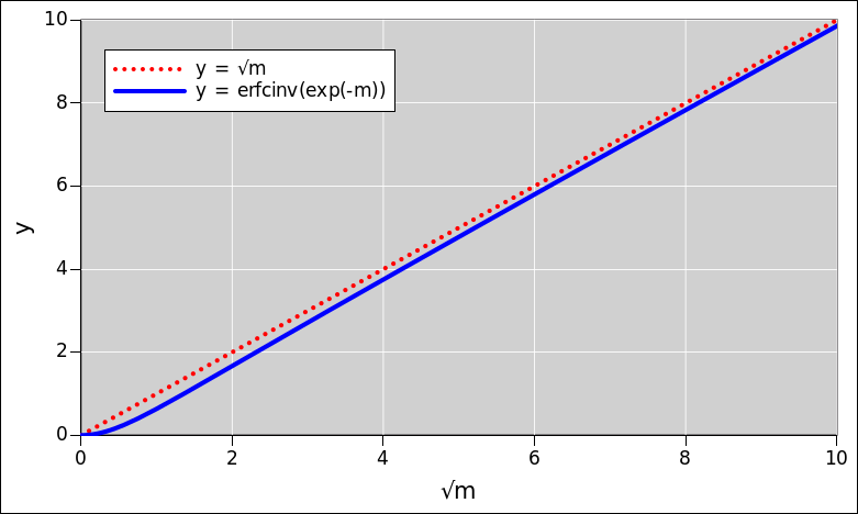
The inverse relationship is:
| (23) |
For m less than 25, we can evaluate equation 23 directly. The function is shown in figure 11
For m greater than 12, we can approximate the erfc to better than 0.1% via:
| (24) |
Taking the logarithm, we get:
| (25) |
We can approximately solve for y in terms of m:
| (26) |
You can see from figure 11 that the y1 approximation is fairly decent. The next iteration (y2) is good enough for all practical purposes.
Combining some more:
| (27) |
where we have made use of the fill factor Φ:
| (28) |
where A is the adamance (in bits) of the raw data, and W is the width (in bits) of the hash codeword.
| (29) |
where y is still considered known as a function of m, hence as a function of r, i.e. as a function of the risk we have decided to tolerate. It’s not a very big number. When the risk is 2−256 i.e. r=256, y is only about 13.3.
So ...
| (30) |
where W is the best the RNG could possibly do. Plugging in an estimate for y gives us
| (31) |
Solve for Φ in terms of the deficit:
| (32) |
If we say we can tolerate a deficit of 0.01 bits, that means there is 255.99 bits of adamance in a 256-bit word. That means the hash-function codeword has 99.996% of the maximum possible adamance. This can be achieved using a fill-factor of about 7.33 million.
Note that 8 million is about 23 bits, so the raw data string needs to have an adamance of at least 256 + 23 = 279 bits. This means the RNG is making reasonably efficient use of the available randomness.
Furthermore, unless the hash function is spectacularly broken, we expect it to be computationally infeasible for the attacker to find or exploit the missing 0.01 bits.
If you add another 7 bits of adamance to the raw data string, it increases the fill-factor by a factor of 128, which knocks the deficit down by an order of magnitude.
By way of analogy, let us consider the relationship between code-breakers and code-makers. This is a complex ever-changing contest. The code-breakers make progress now and then, but the code-makers make progress, too. It is like an “arms race” but much less symmetric, so we prefer the term cat-and-mouse game.
At present, by all accounts, cryptographers enjoy a very lopsided advantage in this game.
There is an analogous relationship between those who make PRNGs and those who offer tools to test for randomness. The PRNG has a hidden pattern. Supposedly the tester “wants” the pattern to be found, while the PRNG-maker doesn’t.
We remark that in addition to the various programs that bill themselves as randomness-testers, any off-the-shelf compression routine can be used as a test: If the data is compressible, it isn’t random.
To deepen our understanding of the testing issue, let’s consider the following scenario: Suppose I establish a web server that puts out pseudo-random bytes. The underlying PRNG is very simple, namely a counter strongly encrypted with a key of my choosing. Each weekend, I choose a new key and reveal the old key.
The funny thing about this scenario is the difference between last week’s PRNG and this week’s PRNG. Specifically: this week’s PRNG will pass any empirical tests for randomness that my adversary cares to run, while last week’s PRNG can easily be shown to be highly non-random, by means of a simple test involving the now-known key.
As a modification of the previous scenario, suppose that each weekend I release a set of one billion keys, such that the key to last week’s PRNG is somewhere in that set. In this scenario, last week’s PRNG can still be shown to be highly non-random, but the test will be very laborious, involving on the order of a billion decryptions.
Note that to be effective against this PRNG, the randomness-testing program will need to release a new version each week. Each version will need to contain the billions of keys needed for checking whether my PRNG-server is “random” or not. This makes a mockery of the idea that there could ever be an all-purpose randomness tester. Even a tester that claims to be “universal” cannot be universal in any practical sense.1 An all-purpose randomness tester would be tantamount to an automatic all-purpose encryption-breaking machine.
To paraphrase Dijkstra: Measurement can prove the absence of entropy, but it cannot prove the presence of entropy. More specifically, a “randomness testing” program will give an upper bound on the entropy density of a random generator, but what we need is a lower bound, which is something else entirely.
The turbid calibration procedure calculates a lower bound on the adamance density, based on a few macroscopic physical properties of the hardware. It is entirely appropriate to measure these macroscopic properties, and to remeasure them occasionally to verify that the hardware hasn’t failed. This provides a lower bound on the entropy, which is vastly more valuable than a statistically-measured upper bound.
As discussed in section 8.5, tests such as Diehard and Maurer’s Universal Statistical Test are far from sufficient to prove the correctess of turbid. They provide upper bounds, whereas we need a lower bound.
When applied to the raw data (at the input to the hash function) such tests report nothing more than the obvious fact that the raw data is not 100% random. When applied to the output of the hash function, they are unable to find patterns, even when the adamance density is 0%, a far cry from the standard (100%) we have set for ourselves.
A related point: Suppose you suspect a hitherto-undetected weakness in turbid. There are only a few possibilities:
The foregoing is a special case of a more general rule: it is hard to discover a pattern unless you have a pretty good idea what you’re looking for. Anything that could automatically discover general patterns would be a universal automatic code-breaker, and there is no reason to believe such a thing will exist anytime soon.
There are some tests that make sense. For instance:
On the one hand, there is nothing wrong with making measurements, if you know what you’re doing. On the other hand, people have gotten into trouble, again and again, by measuring an upper bound on the entropy and mistaking it for a lower bound.
The raison d’etre of turbid is that it provides a reliable lower bound on the adamance density, relying on physics, not relying on empirical upper bounds.
We ran Maurer’s Universal Statistical Test a few times on the output of turbid. We also ran Diehard. No problems were detected. This is totally unsurprising, and it must be emphasized that we are not touting this a serious selling point for turbid; we hold turbid to an incomparably higher standard. As discussed in section 4.2, we consider it necessary but not sufficient for a high-entropy random generator to be able to pass such tests.
To summarize this subsection: At runtime, turbid makes specific checks for common failures. As discussed in section 4.3 occasionally but not routinely apply general-purpose tests to the output.
We believe non-specific tests are very unlikely to detect deficiencies in the raw data (except the grossest of deficiencies), because the hash function conceals a multitude of sins. You, the user, are welcome to apply whatever additional tests you like; who knows, you might catch an error.
We must consider the possibility that something might go wrong with our high entropy random generator. For example, the front-end transistor in the sound card might get damaged, losing its gain (partially or completely). Or there could be a hardware or software bug in the computer that performs that hashing and control functions. We start by considering the case where the failure is detected. (The other case is considered in section 5.2.)
At this point, there are two major options:
We can ornament either of those options by printing an error message somewhere, but experience indicates that such error messages tend to be ignored.
If the throttling option is selected, you might want to have multiple independent generators, so that if one is down, you can rely on the other(s).
The choice of throttling versus concealment depends on the application. There are plenty of high-grade applications where concealment would not be appropriate, since it is tantamount to hoping that your adversary won’t notice the degradation of your random generator.
In any case, there needs to be an option for turning off error concealment, since it interferes with measurement and testing as described in section 4.
We can also try to defend against undetected flaws in the system. Someone could make a cryptanalytic breakthrough, revealing a flaw in the hash algorithm. Or there could be a hardware failure that is undetected by our quality-assurance system.
One option would be to build two independent instances of the generator (using different hardware and different hash algorithms) and combine the outputs. The combining function could be yet another hash function, or something simple like XOR.
Figure 10 can be simplified to
| Source → Digitizer → Hash (33) |
A number of commentators have suggested that the HRNG needs to use a cipher such as DES to perform a “whitening” step, perhaps
| Source → Digitizer → Hash → Whitener (34) |
or perhaps simply
| Source → Digitizer → Whitener (35) |
We consider such whitening schemes to be useless or worse. It’s not entirely clear what problem they are supposed to solve.
Specifically: There are only a few possibilities:
In general, people are accustomed to achieving reliability using the belt-and-suspenders approach, but that only works if the contributions are in parallel, not in series. A chain is only as strong as its weakest link.
In this case, it is a fallacy to think that a whitener can compensate for a weakness in the hash function. As an extreme example, consider the simplest possible hash function, one that just computes the parity of its input. This qualifies as a hash function, because it takes an arbitrary-length input and produces a constant-length output. Now suppose the data-acquisition system produces an endless sequence of symbols with even parity. The symbols have lots of variability, lots of entropy, but always even parity. The output of the hash function is an endless sequence of zeros. That’s not very random. You can run that through DES or any other whitener and it won’t get more random.
As a less extreme example, consider the WEAKHASH-2 function described in section 8.2. The whitener can conceal the obvious problem that all hashcodes have odd parity, but it cannot remedy the fundamental weakness that half the codes are going unused. The problem, no matter how well concealed, is still present at the output of the whitener: half the codes are going unused.
This is easy to understand in terms of entropy: once the entropy is lost, it cannot be recreated.
It is sometimes suggested that there may exist relatively-simple hash functions that have good mixing properties but require a whitener to provide other cryptologic strengths such as the one-way property. We respond by pointing out that the HRNG does not require the one-way property. We recognize that a Pseudo-Random Generator is abjectly dependent on a one-way function to protect its secret internal state, but the HRNG has no secret internal state.
We recognize that the HRNG may have some internal state that we don’t know about, such as a slowly-drifting offset in the data-acquisition system. However, we don’t care. The correctness of the final output depends on the variability in the raw data, via the hash-saturation principle. As long as there is enough unpredictable variability in the raw data, the presence of additional variability (predictable or not) is harmless.
As a practical matter, since the available hash functions are remarkably computationally efficient, it is hard to motivate the search for a “simpler” hash functions, especially if they require whitening or other post-processing.
Finally, we point out that the last two steps in scheme 34 are backwards compared to scheme 36. If you really want whiteness, i.e. good statistical properties, it is better to put the crypto upstream of the contraction.
For some applications, a well-designed PRNG may be good enough. However, for really demanding applications, at some point you might well throw up your hands and decide that implementing a good HRNG is easier.
A typical PRNG, once it has been seeded, depends on a state variable, a deterministic update function, and some sort of cryptologic one-way function. This allows us to classify typical PRNG attacks and failures into the following categories:
The historical record contains many examples of failed PRNGs. For example:
See reference 18 for an overview of ways in which PRNGs can be attacked.
The following scenario serves to illustrate a few more of the ideas enumerated above: Suppose you are building a network appliance. It has no mouse, no keyboard, no disk, and no other easy sources of randomness (unless you use the audio system, or something similar, as described in this document). You want to sell millions of units. They start out identical, except possibly that each one has a network interface with a unique MAC address.
Seeding the PRNG with the MAC address is grossly inadequate. So the only way to have a halfway acceptable PRNG is to configure each unit by depositing into it a unique PRNG state vector. This means that each unit needs a goodly amount of writable but non-volatile storage; it can’t execute out of ROM and volatile RAM alone. Also, the stored state-vector needs to be updated from time to time; otherwise every time the machine is rebooted it will re-use the exact same numbers as last time, which would be an example of failure failure 3. Note that the standard Linux distributions only update the stored seed when the system is given a shutdown command – not if it goes down due to sudden power failure or software crash – which is unacceptable. You have to protect the state vector for all time. In particular, if a rogue employee sneaks a peek at the state vector (either on the machine itself, or on a backup tape, or whatever) and sells it to the adversaries, they can break all the traffic to and from the affected unit(s) from then on, which would be an example of failure failure 2. All these problems can be dealt with, but the cost might be so high that you give up on the PRNG and use a HRNG instead.
A subtle type of improper reseeding or improper stretching (failure 3) is pointed out in reference 19. If you have a source of entropy with a small but nonzero rate, you may be tempted to stir the entropy into the internal state of the PRNG as often as you can, whenever a small amount of entropy (ΔS) becomes available. This alas leaves you open to a track-and-hold attack. The problem is that if the adversaries had captured the previous state, they can capture the new state with only 2ΔS work by brute-force search, which is infinitesimal compared to brute-force capture of a new state from scratch. So you ought to accumulate quite a few bits, and then stir them in all at once (“quantized reseeding”). If the source of entropy is very weak, this may lead to an unacceptable interval between reseedings, which means, once again, that you may be in the market for a HRNG with plenty of throughput, as described in this document.
The Linux kernel random generator /dev/random (reference 20) accumulates entropy in a pool and extracts it using a hash function. It is associated with /dev/urandom which is the same, but becomes a PRNG when the pool entropy goes to zero. Therefore in some sense /dev/urandom can be considered a stretched random generator, but it has the nasty property of using up all the available entropy from /dev/random before it starts doing any stretching. Therefore /dev/urandom provides an example of bad side effects (failure 4). Until the pool entropy goes to zero, every byte read from either /dev/random or /dev/urandom takes 8 bits from the pool. That means that programs that want to read modest amounts of high-grade randomness from /dev/random cannot coexist with programs reading large amounts of lesser-grade randomness from /dev/urandom. In contrast, the stretched random generator described in this document is much better behaved, in that it doesn’t gobble up more entropy than it needs.
It is certainly possible for PRNG failures to be found by direct analysis of the PRNG output, for example by using statistical tools such as reference 21.
More commonly, though, PRNGs are broken by attacking the seed-storage and the seed-generation process. Here are some examples:
If a PRNG contains N bits of internal state, it must repeat itself with a period no longer than 2N. Obviously, N must be large enough to ensure that repetition never occurs in practical situations. However, although that is necessary, it is far from sufficient, and making the period longer is not necessarily a good way to make the PRNG stronger. By way of example: A 4000-bit Linear Feedback Shift Register (LFSR) has a period of 24000 or so, which is a tremendously long period ... but the LFSR can easily be cryptanalyzed on the basis of only 4000 observations (unless it is protected by a strong one-way function installed between the LFSR and the observable output). For a Stretched Random Generator (section 9), it is necessary to have a period long compared to the interval between reseedings, but it is not necessary to make it much longer than that. So, for a SRNG, a huge period is neither necessary nor sufficient. For a PRNG that is not being reseeded, a huge period is necessary but not sufficient.
This is worth emphasizing: One key difference between a genuinely entropic random generator and a pseudo-random generator is that for the PRNG you have to worry about where you get the initial seed, how you recover the seed after a crash/restart, and how you protect the seed for all time, including protecting your backup tapes. For the HRNG you don’t.
See section 1.5.
Attacks against turbid. and similar systems are very different from the usual sort of attack against a PRNG (such as are discussed in section 6.1).
The question is sometimes asked whether thermal noise is really “fundamentally” random. Well, it depends. Obviously, the magnitude of thermal noise depends on temperature, and theoretically an adversary could reduce the temperature of your computer to the point where the input signal calibration was no longer valid. In contrast, there are other processes, such as radioactive decay and quantum zero-point motion, that are insensitive to temperature under ordinary terrestrial conditions. This makes thermal noise in some sense “less fundamental”. However, the distinction is absolutely not worth worrying about. If somebody can get close enough to your computer to radically change the temperature, attacks against the HRNG are the least of your worries. There are other attacks that are easier to mount and harder to detect.
This is a special case of a more-general observation: The most-relevant attacks against the HRNG don’t attack the fundamental physics; they attack later stages in the data acquisition chain, as we now discuss.
Suppose you choose radioactive decay, on the theory that it is a “more fundamentally” random process. The decay process is useless without some sort of data acquisition apparatus, and the apparatus will never be perfect. For one thing, the detector will presumably have live-time / dead-time limitations and other nonidealities. Also, an adversary can interfere with the data acquisition even if the fundamental decay process is beyond reach. Last but not least, the raw signal will exhibit a Poisson distribution, which does not match the flat distribution (all symbols equally likely, i.e. 100% entropy density) that we want to see on the final HRNG output. Therefore the acquired signal will not be one whit more useful than a signal derived from thermal noise. The same sort of postprocessing will be required.
Similar remarks apply to all possible sources of hardware randomness: we do not expect or require that the raw physics will be 100% random; we merely require that it contains some amount of guaranteed randomness.
One very significant threat to the HRNG is the possibility of gross failure. A transistor could burn out, whereupon the signal that contained half a bit of entropy per sample yesterday might contain practically nothing today.
Another very significant threat comes from the possibility of bugs in the software.
Tampering is always a threat; see reference 4 and reference 5.
Even if everything is working as designed, we have to be careful if the noise is small relative to Q, the the quantum of significance of the digitizer, i.e. the voltage represented by least-significant bit.
A more subtle threat arises if the digitizer has “missing codes” or “skimpy codes”. A soundcard that is advertised as having a 24-bit digitizer might really only have a 23-bit digitizer. Most customers wouldn’t notice.
An adversary could mount an active attack. The obvious brute-force approach would be to use a high-power electromagnetic signal at audio frequencies (VLF radio), in the hopes that it would couple to the circuits in the sound card. However, any signal of reasonable size would just add linearly to the normal signal, with no effect on the process of harvesting entropy.
A truly huge signal might overload and saturate the audio input amplifier. This would be a problem for us, because thermal noise would have no effect on an already-saturated output. That is, the small-signal gain would be impaired. An attack of this kind would be instantly detectable. Also, it is likely that if attackers could get close enough to your computer to inject a signal of this magnitude, they could mount a more direct attack. Remember, if we are using a 24-bit soundcard we have almost 16 bits of headroom (a factor of 10,000 or so) between the normal signal levels and the saturation level. I consider an attack that attempts to overload the amplifier so implausible that I didn’t write any code to detect it, but if you feel motivated, you could easily write some code to look at the data as it comes off the data-acquisition system and verify that it is not saturated. Having 16 bits (or more) of resolution is a great luxury. (It would be quite tricky to verify correct operation on other systems that try to get by with only one-bit or two-bit digitizers.)
Another possibility is interference originating within the computer, such as a switching power supply or a video card, that inadvertently produces a signal that drives the sound card into saturation. This is unlikely, unless something is badly broken. Such interference would cause unacceptable performance in ordinary audio applications, at levels very much lower than we care about. A decent soundcard is, by design, well shielded against all known types of interference. That is, a soundcard must provide good performance at low audio levels (little if any discernible additive noise, no matter what interference sources are present) and also good performance at high audio levels (little if any saturation). The possibility that an interference source that is normally so small as to be inaudible would suddenly become so large as to saturate a 24-bit ADC seems quite insignificant, unless there is a gross hardware failure. The odds here are not dominated by the statisics of the noise processes; they are dominated by the MTBF of your hardware.
Even if there is no interference, it may be that the sound card, or the I/O bus, radiates some signal that is correlated with the raw data that is being provided to the program. However, if you are worried about this sort of passive attack you need to be worried about compromising emanations (TEMPEST) from other parts of your system also. See reference 22. There is no reason to believe the audio hardware or HRNG software unduly increases your vulnerability in this area.
The least-fundamental threats are probably the most important in practice. As an example in this category, consider the possibility that the generator is running on a multiuser machine, and some user might (inadvertently or otherwise) change the mixer gain. To prevent this, we went to a lot of trouble to patch the ALSA system so that we can open the mixer device in “exclusive” mode, so that nobody else can write to it.
We do not need the samples to be completely independent. All we need is some independence.
Here’s an example that may help explain how this works.
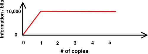
Suppose I select 2500 completely random hex digits and write them on a page of blue paper. The ensemble of similarly-prepared pages has 10,000 bits of entropy. I copy the digits onto a page of red paper, and send you one of the pages.
The page gives you 10,000 bits of information that you didn’t have previously. After you look at the page, the entropy of the ensemble goes to zero.
If I now send you the other page, it conveys zero addtional information. This demonstrates than information and entropy are not extensive variables. This is illustrated in figure 12. A lot of introductory chemistry books will tell you that energy and entropy are extensive, but reality is more complicated – for both energy and entropy – especially for smallish systems where the surface makes a nontrivial contribution.
What’s even more amusing is that it doesn’t matter which page I send first (red or blue) – the first one conveys information but the second one does not.
It is possible for a source to be partially dependent and partially independent. For example, suppose we shuffle a deck of cards. The ensemble of such decks has slightly more than 225 bits of entropy. That’s log2(52!). As is customary, this assumes we pay attention only to suit and rank, not orientation or anything like that.
Now we take ten copies of that deck, all ordered alike. At this stage they are 100% dependent. Then we “cut the deck” randomly and independently. “Cutting” means applying one of the 52 different full-length permutations. Now, the first deck we look at will provide 225 bits of entropy, and each one thereafter will provide 5.7 bits of additional entropy, since log2(52)=5.7. So in this situation, each deck can be trusted to provide 5.7 bits of entropy.
In this situation, requiring each deck to have no dependence on the others would be an overly strict requirement. We do not need full independence; we just need some independence, as quantified by the provable lower bound on the entropy. To repeat: we don’t need to quantify how much dependence there is; we just need to quantify how much independence there is. In our example, there is provably at least 5.7 bits of usable entropy per deck.
If you wanted, you could do a deeper analysis of this example, taking into account the fact that the entropy we are relying on, 5.7 bits, is not the whole story. We can safely use 5.7 bits as a lower bound, but under some conditions more entropy is available, as can be quantified by considering the joint probability distribution and computing the entropy of that distribution. Meanwhile the fact remains that we are not required to extract every last bit of available randomness. Under a wide range of practical conditions, it makes sense to engineer a random generator based on provable lower bounds, since that is good enough to get the job done, and a deeper analysis would not be worth the trouble.
For a typical personal workstation, the demand for high-grade randomness is quite nonuniform. The average demand is rather modest, but the peak demand can be considerably higher. Uses include:
For such uses, I/O timing typically provides a perfectly adequate supply of entropy. The Linux kernel random generator is an example: it collects a few bits per second from timing mouse, keyboard, and disk events.
Servers are more problematic than workstations. Often they have a much greater demand for entropy, and less supply. An example is a server which terminates hundreds of IPsec tunnels. During start-up it requires more than a hundred thousand high-quality random bits in a short time, which is far more than can be buffered in /dev/random, and far more than can be collected by the kernel in the available time.
An even worse situation arises in small networked controllers, which have no mouse, no keyboard, no disk, nor any other good sources of entropy. If we want to establish secure IPsec or ssh connections to such boxes, we simply must come up with a source of entropy.
Similarly, virtual machines need randomness but might not have any good way of obtaining it.
At this point, one often hears the suggestion that we send the box some new entropy over the network. This is not a complete solution, because although it helps defend against certain threats, it leaves others undefended. One problem is that if security is compromised once (perhaps because somebody stole the PRNG seed) then security is compromised more-or-less forever, because the adversary can read the network traffic that carries the new entropy.
The sound card can produce quite a bit of entropy. Even a low-end sound card can produce 44,000 bits per second. A Delta-1010 (which has a higher sample rate, higher resolution, and more channels) can produce a couple million bits per second.
In order for the HRNG to work, the hash function be reasonably well-behaved. As an example of what could go wrong, consider a few badly-behaved examples:
Weak hash functions have the property that they waste entropy. That is, their outputs are in some way more predictable than the outputs of a strong hash function would be. Obviously for our purposes we want to use a strong hash function.
The hash function cannot possibly create entropy, and we do not need it to do so. Instead, what we need is a hash function that does not waste entropy through unnecessary hash collisions. In the unsaturated regime, there should be very few collisions, so any entropy present at the input is passed to the output without loss. In the saturated regime, when the output approaches 100% entropy density, there will necessarily be collisions and loss of entropy.
Hash functions are used in a wide range of applications. As a first example, let us consider how hash functions are used in compilers: the input to the hash function is a symbol-name, and the output is used as an index into the symbol table. It is often much more efficient to manipulate the hash than to manipulate the corresponding input string.
When two different inputs produce the same hash, it is called a hash collision. This is not desirable from the compiler’s point of view. So, the essential properties of a compiler-grade hash function are:
- 1) It takes as input a variable-length string, and returns a fixed-length string, called the hash.
- 2) It is a function; that is, the same input produces the same output every time.
- 3) Vague anti-collision property: There should not be more hash collisions than necessary.
A cryptologic hash function has several additional properties:
- 4) Noninvertibility: For any given hash, it is is computationally infeasible to find an input that generates that hash.
- 5) Cryptologic anti-collision property: It is computationally infeasible to construct two different inputs that produce the same hash.
A typical application for a cryptologic hash is to compute a Hashed Message Authentication Code (HMAC), which can be used to detect and deter tampering with the message. See reference 23.
Property #4 (noninvertibility) only applies if there is a sufficient diversity of possible inputs. If the only possible inputs are “yes” and “no” then the adversary can easily search the input space; this is called a brute-force attack. When computing HMACs one prevents such a search by padding the message with a few hundred bits of entropy. The hash function itself has property #2 but not property #4, while the HMAC has property #4 but not property #2, because HMAC(message) = HASH(padding+message).
When building a High-Entropy Random Generator, we do not require noninvertibility at all. If the adversary knows the current hash-function output, we don’t care if the hash-function input can be inferred, because that has no bearing on any past or future outputs. The generator has no memory. This is one of the great attractions of this HRNG design, because nobody has ever found a function that is provably noninvertible.
In stark contrast, noninvertibility is crucial for any Pseudo-Random Generator. It is easy to arrange that the state variable (the input to the hash function) has plenty of bits, to prevent brute-force searching; that’s not the problem. The problem lies in initializing the state variable, and then defending it for all time. The defense rests on the unproven assumption that the hash function is noninvertible. What’s worse, the burden on the hash function is even heavier than it is in other applications: The hash function must not leak even partial information about its input. Otherwise, since the hash function is called repeatedly, the attacker would be able to gradually accumulate information about the generator’s internal state.
In discussions of this topic, the following notion often crops up:
- 6) Strict avalanche2 property: whenever one input bit is changed, every output bit must change with probability ½. See reference 24.
This statement is not, alas, strict enough for our purposes. Indeed, WEAKHASH-1 and WEAKHASH-2 satisfy this so-called strict avalanche criterion. To be useful, one would need to say something about two-bit and multi-bit changes in the input. We dare not require that every change in the input cause a change in the output, because there is a simple pigeon-hole argument: There are V = 2562100 input states and only C = 2160 output states. There will be hash collisions; see section 3.4.
To see what criteria are really needed, we will need a more sophisticated analysis. The most general representation of a hash function (indeed any function) is as a function table. Table 2 shows a rather weak hash function.
| Row | Input | Output |
| 1 | () | (01) |
| 2 | (0) | (10) |
| 3 | (1) | (11) |
| 4 | (00) | (00) |
| 5 | (01) | (01) |
| 6 | (10) | (10) |
| 7 | (11) | (11) |
| 8 | (000) | (00) |
| 9 | (001) | (01) |
| 10 | (010) | (10) |
| 11 | (011) | (11) |
| 12 | (100) | (00) |
| 13 | (101) | (01) |
| 14 | (110) | (10) |
| 15 | (111) | (11) |
The input symbols are delimited by parentheses to emphasize that they are variable-length strings; row 1 is the zero-length string. It should be obvious how to extend the table to cover arbitrary-length inputs. It should also be obvious how to generalize it to larger numbers of hashcodes.
The hashcodes in the Output column were constructed by cycling through all possible codes, in order. All possible codes occur, provided of course that there are enough rows, i.e. enough possible inputs. What’s more, all possible codes occur with nearly-uniform frequency, as nearly as can be. This construction produces exactly uniform frequency if and only if the number of rows is a multiple the number of possible codes, which we call the commensurate case. The example in the table is non-commensurate, so even though the codes are distributed as evenly as possible, complete evenness is not possible. In this example, the (00) code is slightly underrepresented.
Table 2 is a hash function in the sense that it maps arbitary-length inputs to fixed-length outputs, but it has very poor collision-resistance, and it has no vestige of one-wayness.
Starting from table 2 can construct a better hash function by permuting the rows in the Output column, as shown in table 3. If there are R rows in the table and C possible codes, there are V! / (V/C)!C distinct permutations. This is exact in the commensurate case, and a lower bound otherwise. This is a huge number in practical situations such as V = 2562100 and C = 2160.
| Row | Input | Output |
| 1 | () | (01) |
| 2 | (0) | (10) |
| 3 | (1) | (10) |
| 4 | (00) | (00) |
| 5 | (01) | (11) |
| 6 | (10) | (01) |
| 7 | (11) | (01) |
| 8 | (000) | (11) |
| 9 | (001) | (10) |
| 10 | (010) | (00) |
| 11 | (011) | (11) |
| 12 | (100) | (00) |
| 13 | (101) | (11) |
| 14 | (110) | (01) |
| 15 | (111) | (10) |
If we temporarily assume a uniform probability measure on the set of all possible permutations, we can choose a permutation and use it to construct a hash function. Statistically speaking, almost all hash functions constructed in this way will have very good anti-collision properties and one-way properties (assuming V and C are reasonably large, so that it makes sense to make statistical statements).
This way of constructing hash functions is more practical than it might initially appear. Note that any cipher can be considered a permutation on the space of all possible texts of a given length. Hint: use a pigeon-hole argument: The ciphertext is the same length as the plaintext, and the fact that the cipher is decipherable guarantees that there is a one-to-one correspondence between ciphertexts and plaintexts.
This suggests a general method of constructing hash functions: Pad all intputs to some fixed length. Append a representation of the original length, so that we don’t have collisions between messages that differ only in the amount of padding required. Encipher. If it’s a block cipher, use appropriate chaining so that the resulting permutation isn’t a block-diagonal matrix. Pass the cipertext through a contraction function such as WEAKHASH-0 to produce a fixed-length output. That is:
| Pad → Encipher → Contract (36) |
For starters, this serves to answer a theoretical question: it is certainly possible for a hash function to generate all codes uniformly.
By the way, a hash constructed this way will have the one-way property, if the adversaries don’t know how to decipher your cipher. You could ensure this by using a public-key cipher and discarding the private key. (For what it’s worth, if you don’t need the one-way property, you could even use a symmetric cipher without bothering to keep the key secret.)Another way to add the one-way property, for instance for a PRNG or SRNG, is to tack on a one-way function downstream of the cipher-based hash function. This may be more computationally efficient than using asymmetric crypto. A cipher with a random key will suffice. If the one-way function requires a key, consider that to be part of the keying and re-keying requirements of the PRNG or SRNG.
In any case, keep in mind that turbid does not require its hash to be one-way.
We remark that many modern hash functions including SHA-256 follow the general plan Pad → Scramble → Contract which is rather similar to scheme 36. A key difference is that the scramble function is not a normal cipher, because it is not meant to be deciphered. The Feistel scheme is conspicuously absent. Therefore we can’t easily prove that it is really a permutation. The pigeon-hole argument doesn’t apply, and we can’t be 100% sure that all hashcodes are being generated uniformly.
In section 8.3 we temporarily assumed a uniform distribution on all possible truth-tables. That’s not quite realistic; the mixing performed by any off-the-shelf hash function is not the same as would be produced by a randomly-chosen function table. We need to argue that it is, with virtual certainty, impossible for anyone to tell the difference, even if the adversaries have unlimited computing power.
Rather than just assuming that the hash function has the desired property, let’s look a little more closely at what is required, and how such a property can come about.
In section 8.3 each row in the Input column was treated pretty much the same as any other row. It is better to assign measure to each input-state according to the probability with which our data-acquisition system generates that state.
We then sort the truth-table according to the probability of each input. (This sort keeps rows intact, preserving the Input/Output relationship, unlike the permutation discussed previously which permuted one column relative to the others.) In the Input column we list all the states (all 2562100 of them) in descending order of probability. In the Output column we find the corresponding hash. This allows us to see the problem with WEAKHASH-1: Because we are imagining that the data is an IID sequence of samples, with much less than 100% adamance density, a huge preponderance of the high-probability data strings will have the same hash, because of the permutation-invariance. Certain hashcodes will be vastly over-represented near the top of the list.
So we require something much stronger than the so-called strict avalanche property. Mainly, we require that anything that is a symmetry or near-symmetry of the raw data must not be a symmetry of the hash function. If single-bit flips are likely in the raw data, then flipping a single bit should move the data-string into a new hashcode. If flipping a few bits at a time is likely, or permutations are likely, then such things should also move the data-string to a new hashcode.
The input buffer will typically contain some bits that carry little or no entropy. In the space of all possible function tables, there must exist some hash functions that look at all the wrong bits. However, these must be fantastically rare. Consider the cipher-based hash functions decribed previously. For almost any choice of cipher key, the function will permute the hashcodes so that a representative sample falls at the top of the list. The key need not be kept secret (since the adversaries have no power to change the statistics of the raw data).
Unless we are extraordinarily unlucky, the symmetries of natural physical processes are not symmetries of the hash function we are using.
Let us contrast how much a cryptologic hash function provides with how little we need:
| A cryptologic hash function advertises that it is computationally infeasible for an adversary to unmix the hashcodes. | What we are asking is not really very special. We merely ask that the hashcodes in the Output column be well mixed. |
| A chosen-plaintext (chosen-input) attack will not discover inputs that produce hash collisions with any great probability. | We ask that the data acquisition system will not accidentally produce an input pattern that unmixes the hashcodes. |
We believe that anything that makes a good pretense of being a cryptologic hash function is good enough for our purposes, with a wide margin of safety. If it resists attack when the adversary can choose the inputs, it presumably resists attack when the adversary can’t choose the inputs. See also section 8.5.
Note that we don’t care how much the adversary knows about the distribution from which the input samples are drawn. We just need to make sure that there is enough sample-to-sample variability. If there is some 60-cycle hum or other interference, even something injected by an adversary, that cannot reduce the variability (except in ultra-extreme cases).
Once noise is added to a signal, it is very hard to remove — as anyone who has ever tried to design a low-noise circuit can testify.
It is often suggested that we test whether the output of turbid is random, using packages such as Diehard (reference 25) and Maurer’s Universal Statistical Test (“MUST”, reference 21). We have several things to say in response:
- 1) SHA-256 does pass those tests.
- 2) SHA-256 passes an even stricter test, namely the counter test described below.
- 3) Being able to pass such a test is necessary but far from sufficient as a criterion for the correctness of the turbid program. See section 4.
We note in passing a trivial weakness: There is a wide category of hash functions (including SHA-256), each of which operates on blocks of input data, and are Markovian in the sense that they remember only a limited amount of information about previous blocks. It has been shown that any hash in this category will be more vulnerable to multicollisions than an ideal hash would be. However, this is a chosen-plaintext attack, and is not even remotely a threat to turbid.
SHA-256 has been cryptanalyzed by experts; see e.g. reference 26 and reference 27. To date, no attacks have been reported that raise even the slightest doubts about its suitability for use in turbid.
However, bowing to popular demand, we performed some tests, as follows: We constructed a 60-bit counter using the LSB from each of 60 32-bit words; the higher 31 bits of each word remained zero throughout. These sparsely-represented 60-bit numbers were used, one by one, as input to the hash function. The resulting hashcodes were taken as the output, analogous to the output of turbid. We then applied Diehard and MUST.
As expected, SHA-256 passed these tests. Even the older, weaker SHA-1 passed these tests. Such tests are more likely to catch coding errors than to catch weaknesses in the underlying algorithm, when applied to professional-grade algorithms.
In relative terms, we consider this counter-based approach to be in some ways stricter than testing the output of turbid under normal operating conditions, because the counter has zero entropy. It has a goodly number of permanently-stuck bits, and the input to the hash function changes by usually only one or two bits each time.
However, in absolute terms, we consider all such tests ludicrously lame, indicative of the weakness of the tests, not indicative of the strength of SHA-256. We don’t want turbid to be judged by such low standards. See section 4 for more on this.
The turbid program comes bundled with a Stretched Random Generator. Its adamance density is strictly greater than zero but less than 100%. To use it, read from /dev/srandom.
The SRNG seeds itself, and reseeds itself every so often, using entropy from the HRNG. Reading from /dev/srandom consumes entropy 10,000 times more sparingly than reading from /dev/hrandom or /dev/random or /dev/urandom. It is also less compute-intensive than /dev/urandom.
The principle of operation is as follows: In addition to the seeding/reseeding process, there is a state variable, a deterministic update function, and a hash function. Between reseedings, at each iteration we deterministically update the state variable and feed it to the hash function. The output of the hash function is the output of the SRNG.
The update function treats the state variable as three 32-bit registers. Each register has a random starting point. The first register is updated by adding a random odd addend. The second is a Linear Feedback Shift Register. The third is another LFSR, with a different period. (This design was chosen because each register can be separately tested, in contrast to one big 96-bit LFSR which would be harder to test.) Each register separately has a period on the order of 232 and combined they give a period on the order of 296. The period is billions upon billions of times longer than it needs to be, because after 10,000 iterations the state variable is strongly perturbed using 128 bits of pure entropy from the HRNG.
It is commonly assumed that having a super-long period is a hallmark of a good PRNG. However, that’s neither necessary nor sufficient. A 4000-bit LFSR has a period of 24000 or so, but it can easily be cryptanalyzed on the basis of only 4000 observations (unless it is protected by a strong one-way function installed between the LFSR and the observable output). It is necessary to have a period long compared to the interval between reseedings, but it is not necessary to make it much longer than that. In summary, if the period is long enough, making it longer confers no advantage.
Unlike the HRNG, the SRNG must assume that the hash function has the one-way property. That is, we assume an adversary (even after ∼10,000 observations of the output of the hash function) cannot infer anything useful about the state variable.
The defining property of a SRNG is that it has an average entropy density that is greater than zero but less than 100%. Let’s take a moment to discuss where in the output-stream this entropy is to be found. Suppose you have 1024 bits of entropy available for seeding your generator, which you then use to put out a very long output string.
For a discussion of the Fortuna class of random generators, and how that contrasts with turbid, see reference 28.
For a discussion of the Linux device driver for /dev/random and /dev/urandom, see reference 20.
There is a vast literature on hash functions in general. Reference 24 is a starting point. Reference 29 is a useful literature survey. Reference 30 was an influential early program for harvesting entropy from the audio system; it differs from turbid in not having calibration features. Reference 31 uses the physics of a spinning disk as a source of entropy.
Methods for removing bias from a coin-toss go back to von Neuman; see reference 32 and references therein; also reference 33.
Reference 34 suggests hashing 308 bits (biased 99% toward zero) and taking the low-order 5 bits of the hash to produce an unbiased result. This is correct as far as it goes, but it is inefficient, wasting 80% of the input entropy. Presumably that reflects an incomplete understanding of the hash-saturation principle, in particular the convergence properties discussed in section 3.4, which would have led immediately to consideration of wider hashcodes. There is also no attempt to quantify how nearly unbiased the result is.
Thanks to Steve Bellovin, Paul Honig, and David Wagner for encouragement, incisive questions, and valuable suggestions.
Practical sources of randomness can be characterized in terms of the adamance density. The raw sources have an adamance density greater than zero and less than 100%. The methods disclosed here make it possible to produce an output that approaches 100% adamance density as closely as you wish, producing symbols that are random enough for any practical purpose. It is important to have a calculated lower bound on the adamance density. In contrast, statistical tests provide only an upper bound, which is not what we need.
It is possible to generate industrial-strength randomness at very low cost, for example by distilling the randomness that is present in ordinary audio interfaces.
In order to refine our notions of what is random and what is not, consider the following million-character strings. We start with
That seems distinctly non-random, very predictable, not very complex. Next, consider the string
That seems also non-random, very predictable, not very complex.
That is somewhat more interesting. The digits pass all known tests for randomness with one narrow exception (namely tests that check for digits of π). However, they must still be considered completely predictable. Finally, consider the two strings
The million-character string represented by example E5 is, as far as anybody knows, completely random and unpredictable. Example E4 is very similar, except that the letter “A” appears more often than it would by chance. This string is mostly unpredictable, but contains a small element of nonrandomness and predictability.
Following Solomonoff (reference 35 and reference 36) and Chaitin (reference 37) we quantify the surprisal of a string of symbols as follows:
Let z be a string of symbols. The elements of z are denoted zk and are drawn from some alphabet Z. The number of symbols in the alphabet is denoted #Z.
Let PC(z) be the probability that computer programs, when run on a given computer C, will print z and then halt. The surprisal is defined to be the negative logarithm of this probability, denoted $C(z) := − logPC(z). In this document we choose to use base-2 logarithms, so that surprisal is measured in bits. Surprisal is also known as the surprise value or equivalently the unexpectedness. It is intimately related to entropy, as discussed below.
Note that we are using one probability distribution (the probability of choosing a computer program) to derive another (the probability PC(z) of a symbol string). To get this process started, we need to specify a method for choosing the programs. Better yet, using the notions of measure theory, we realize that probability need not involve choosing at all; instead all we really need is a method for assigning weight (i.e. measure) to each of the possible programs. Here is a simple method:3 Consider all possible programs of length exactly L* (measured in bits, since we are representing all programs as bit-strings). Assign each such program equal measure, namely 2−L*. Then test each one and count how many of them produce the desired output string z and then halt, when run on the given computer C. The measure of a string is the total measure of the set of programs that produce it. A string that can be produced by many different programs accumulates a large probability.
In this construction, a short program X (i.e. one which has a length L(X) less than L*) is not represented directly, but instead is represented by its children, i.e. programs formed from X by padding it with comments to reach the required length L*. There are at least 2L*−L(X) ways of doing the padding, and each way contributes 2−L* to the total measure. This means that a string z that can be produced by a short programs X will have a probability at least 2−L(X), no matter how large L* is. We take the limit as L* becomes very large and use this in the definition of PC(z).
Usually the probability PC(z) is dominated by (the children of) the shortest program that produces z. Therefore some people like to use the length of this shortest program as an estimate of the surprisal. This is often a good estimate, but it should not be taken as the definition.
The explicit dependence of PC(z) on the choice of computer C calls attention to an element of arbitrariness that is inherent in any definition of surprisal. Different people will assign different values to “the” surprisal, depending on what resources they have, and on what a priori information they have about the situation.
In an adversarial situation such as cryptography, we suggest that probabilities be defined in terms of the adversary’s computer. If you have multiple adversaries, they can be treated as a single adversary with a parallel computer.
In this section, for conciseness, we drop the subscript C ... but you should remember that the probabilities and related quantities are still implicitly dependent on the choice of C.
A relatively minor objection to this definition of surprisal is that PC(z) includes contributions from arbitrarily-long programs. That is a problem in theory, but in practice the sum is dominated by relatively short programs, and the limit converges quickly.
A much more serious objection is that even for modest-sized programs, the definition runs afoul of the halting problem. That is, there may well be programs that run for a million years without halting, and we don’t know whether they would eventually produce string z and then halt. This means the surprisal, as defined here, is a formally uncomputable quantity.
We will duck both these issues, except for the following remarks.
In this section we shift attention from the unpredictability of strings to the unpredictability of the individual symbols making up the string.
Let us re-examine the examples given at the beginning of this section. Example E5 has surprisal $(z) very close to L(z) log(#Z). We classify strings of this sort as absolutely-random, by which we mean algorithmically-random.
Examples E1, E2, and E3 all have surprisal much less than their length. These strings are clearly not absolutely-random.
The interesting case is example E4. Intuitively, we think of this as “somewhat unpredictable” but more predictable than E5. To make this notion quantitative, we introduce the notion of surprise density. The following quantity tells us the surprise density of the string z in the region from i to j:
| σj|i(z) := |
| (37) |
where Front(z,i) is the substring formed by taking the first i symbols of the string z.
The surprise density for examples E1, E2, and E3 is zero for any region not too near the beginning. The surprise density for example E5 is as large as it possibly could be, namely 100% of log(#Z). Example E4 illustrates the interesting case where the surprise density is quite a bit greater than zero, but not quite 100% of log(#Z).
As mentioned in section 1.2, we consider the unadorned term “random” to be ambiguous, because it means different things to different people. Some people think “random” should denote 100% surprise density, and anything less than that is “non-random” even if it contains a great deal of unpredictability. Other folks think that “random” refers to anything with an surprisal density greater than zero, and “non-random” means completely predictable. Yet other folks extend “random” to include pseudo-random strings, as long as they are “random enough” for some application of interest. Even some professionals in the field use the word this way; reference 38 and the more recent reference 39 speak of “deterministic random number generators”, although it could be argued that it is impossible in principle for a process to be both deterministic and random. The randomness of a PRNG comes from the seed. Calling a PRNG “deterministic” seriously understates the importance of the seed. Compare reference 40.
In the space of all possible strings, almost all strings are absolutely-random, i.e. are algorithmically-random, i.e. contain 100% surprise density. However, the strings we find in nature, and the strings we can easily describe, all have very little surprise density. We can summarize this by saying: “All strings are absolutely-random, except for the ones we know about”.
We can use similar ideas to describe PRNGs and contrast them with HRNGs.
| Most of modern cryptography revolves around notions of computational intractability. (I’m not saying that’s good or bad; it is what it is. | In contrast, there is another set of notions, including entropy and the related notion of unicity distance, that have got nothing to do with computational intractability. |
| The long strings produced by a good PRNG are conditionally compressible in the sense that we know there exists a shorter representation, but at the same time we believe them to be conditionally incompressible in the sense that the adversary has no feasible way of finding a shorter representation. | The long strings produced by a HRNG are unconditionally, absolutely incompressible. Specifically, the set of strings collectively cannot be compressed at all. As for each string individually, it is not compressible either, except possibly for trivially rare cases and/or trivial amounts of compression. |
In this section we climb down a bit from the formality of the previous section.
Let C be a machine that endlessly emits symbols from some alphabet Z. We assume the symbols are IID, that is, independent and identically distributed. That means we can calculate things on a symbol-by-symbol basis, without worrying about strings, the length of strings, or any of that. Let PC(i) denote the probability of the ith symbol in the alphabet.
Note: Nothing is ever exactly IID, but real soundcards are expected to be very nearly IID. At the least, we can say that they are expected to have very little memory. What we require for good random generation is a very mild subset of what is required for good audio performance.
The surprisal of a given symbol is
| $C(i) := log(1/PC(i)) (38) |
By extension we can talk about the probability of a string of symbols. Since the symbols are IID, the probability of a string z is:
| PC(z) := |
| PC(zk) (39) |
where zk is the symbol in the kth position in the string. As an immediate corollary,
| $C(z) := |
| $C(zk) (40) |
which just says that the surprisal is additive in a nice way.
The source entropy of the machine C is defined to be:
| SC := |
| PC(i) log(1/PC(i)) (41) |
Let’s be clear: The surprisal is a property of the symbol, while the entropy is a property of the source. In particular, the entropy is the appropriately-weighted average surprisal.
For a long string, we expect the surprisal of the string to converge to the entropy of the source times the length of the string. The probability of this happening converges to 1, as the string gets longer and longer.
Beware: In the literature it is common to see the word “entropy” used in places where some other quantity would make more sense. In terms of Rényi functionals, sometimes H1 (the plain old entropy) is appropriate, sometimes H∞ is appropriate, and sometimes both or neither.
As a partially-related point: The Linux /dev/random driver keeps track of the “amount of entropy” in the “pool” (i.e. buffer). That idea is in the right general ballpark, but some remarks are in order:
In general the attacker can work in a two-dimensional space. The variables are how much does it cost to break a message of a particular type, and the probability of seeing such a message. The attacker can sit wherever he likes in this space, depending on whether he wants a quicker break or a cheaper break. He can make the tradeoff however he likes.
Let’s analyze this from the sender’s point of view, to see how he would defend against this. We make the task more challenging by assuming that a great many messages are sent. The attacker can apply his best guess to each message, and then move on to the next message. He never needs to bother with his second-best guess.
The sender can draw samples from the orignal (skewed) distribution, and can concatenate them to produce a new (less-skewed) distribution. Subject to the given threat model, the thing we care about is entirely dominated by the most-likely element of the distribution. That is, the distribution in figure 5 there is only 1 bit of adamance per sample, even though there are 4 bits of entropy per sample.
The source entropy S in equation 2b is a single number that characterizes the “average” behavior of the source. For a small sample from a highly-skewed distribution, S doesn’t tell you everything you need to know. This doesn’t change the definition of entropy; entropy is always defined by equation 2b. It just means that equation 2b by itself doesn’t solve all the world’s problems.
Within the given threat model, we are better off looking at H∞, the Rényi functional of order α. It is numerically equal to the surprisal of the most-probable element of the distribution.
In practice, turbid doesn’t have too much of a problem with skewed distributions, for two reasons: First of all, the raw data from a typical soundcard is not terribly skewed. It could perhaps be skewed if the card is producing much less than 1 bit of entropy per sample ... but such cards produce so little randomness that your best strategy is to go buy a better card.
As a warm-up exercise, let’s consider the case of a one-bit digitizer – i.e. a comparator – applied to Gaussian noise. The probabilities are shown in figure 13. Assuming the threshold of the comparator is fixed at zero, the any input in the reddish-shaded region will result in a “low” output, while any input in the bluish-shaded region will result in a “high” output.
Assuming the samples are IID, the entropy per sample coming out of the comparator is
| (42) |
| (43) |
A plot of equation 42 is shown by the blue curve in figure 14. It should be obvious by symmetry that the entropy is one bit per sample when the Gaussian is centered at zero. The case where µ/σ=0.5 (the case illustrated in figure 13), the entropy is 0.79 bits.
Minor tangential remark: We know by looking at its definition that the entropy-versus-offset curve cannot possibly be a Gaussian, but it is astonishingly close.
As always, turbid is designed around provable lower bounds on the entropy. Since we cannot be certain where the Gaussian sits relative to the nearest riser, we assume the worst case, namely that it sits in the middle of a tread. In practice this doesn’t cost us much, because it produces a fairly tight lower bound. The bound stops being tight when σ/Q is quite small (less than 0.2 or so), which only happens when the soundcard has too little sensitivity for practical use.
Example: The Line-In port on the Thinkpad 600 is woefully lacking in sensitivity, and its impedance and bandwith are unimpressive also. As a consequence, it has a rather narrow Gaussian which could easily sit entirely (except for negligible wings) in the middle of a single tread, so we cannot derive a useful lower bound on the entropy. Although intuition suggests that the signal actually contains some entropy, we can’t prove it, so we give up on this port. We use the Mike-In port instead, which has vastly more sensitivity.
Let’s take the next step in developing the ideas. the A-to-D system has three output codes, not just two. Let Q denote the spacing between codes. In other words, Q is the width of a tread.
Terminology: Figure 15 shows the transfer function for an ideal voltmeter. A function that looks like this is called a staircase function, for obvious reasons. In this example, the resolution is 1 microvolt. Any analog input in the open interval (−2.5, 2.5) microvolts will produce a digital reading of 2 microvolts. This corresponds to a horizontal piece of the transfer function. Any such horizontal piece is called a tread, borrowing a term from the architecture of real staircases.Meanwhile, in the graph, the vertical line that connects one tread to the next is called a riser. The riser is not part of the definition of the function, but we can draw it anyway, as a guide to the eye. More precisely, we will use the same word – riser – to refer to the input voltage where the output changes discontinuously from one code to another. At such points, we care more about the input voltage than the output code. No matter how (or whether) you define the transfer function at this point, it will be discontinuous at each riser.
Figure 16 shows the probabilities, assuming Q=1 for simplicity. (In practice Q is on the order of a nanovolt or a microvolt, not a whole volt.)
The equation for the entropy now has three terms, not just two:
| (44) |
| (45) |
For a reasonably wide Gaussian, using three codes allows us to obtain more than one bit per sample. The best case is when the Gaussian is centered in the middle of a tread, as you can see in figure 17.
We now consider the case of a narrow Gaussian, being centered on a tread is the worst case, from the defenders’ point of view, as you can see in figure 19. Only the one code gets generated with any appreciable probability. If we shift the narrow Gaussian so that it straddles a riser, we know we can get one bit per sample, as discussed in section C.1.
Nobody in the real world uses a three-code digitizer. However, it was worth deriving equation 44, because it provides a three-term approximation that is useful whenever the voltage distribution is narrow. That’s because even if the digitizer has many levels, when the distribution is narrow, only three of the codes make any significant contribution.
We can examine this as a function of σ. When the Gaussian is centered on a riser, when σ is near 1.1608, the three-code digitizer does as well as it could possibly do. That’s the point where ½erf(0.5/σ √2) is equal to one third. So all three codes are generated with equal probability. The horizontal black reference line in figure 20 represents one trit. That’s the same as log2(3) bits, i.e. just less than 1.6 bits.
At this special point, when all three codes are equiprobable, the adamance is equal to the entropy.
When σ is half of Q, we are still getting about 1 bit per sample, which is not great, but not terrible. Even when σ is 1/4 of Q, and the Gaussian is centered on a tread, we get 0.3 bits per sample, but things go rapidly to pot after that. When σ is 1/8th of Q, we are getting only 0.001 bits per sample, which is usually not worth the trouble.
In principle, if the Gaussian were centered on a riser, it would produce one bit of entropy and one bit of adamance per sample, even when the width σ was very small. However, it would not be easy to guarantee that the Gaussian was always sufficiently well centered.
Fortunately, it is easy to find soundcards where the RMS voltage is very large compared to Q. In that case, the three-term approximation discussed in this section is not valid and not needed.
Let’s consider the case where the digitizer produces thousands of different codes, and the input distribution is very wide compared to the width of a tread. Let the width of each tread be denoted Q. Equation 44 generalizes as follows:
| (46) |
There will be a discrete amount of probability Pi associated with each tread, i.e. with each digitizer code. The situation is shown in figure 21. The highlighted area represents one of the Pi terms that contributes to the sum in equation 46.
In the limit where the width of the distribution σ is large compared to the digitizer step Q, the Pi inside the logarithm in equation 46 can be simplified. We approximate the integral by height times width.
| (47) |
The explicit factor of log(e) is necessary, because the logarithms in these equations could use any base. [If I had wanted to specify the natural logarithm, I would have written ln() instead of log().] In particular, you might well want to use base-2 logarithms, so that the entropy comes out measured in bits.
The first term inside the square brackets in equation 47 is independent of i, so it can be summed immediately.
To handle the other term, we make another approximation. In the limit, the V inside the integral is never very different from i2Q2, so we can bring the latter inside the integral. So at this point we have
| (48) |
The definite integral inside the big square brackets is easy to do. It is equal to 1/2. So, all that work leaves us with a remarkably simple expression for the entropy per sample:
| (49) |
The first term is easy to understand in terms of dimensional analysis – just ask how many bins fall under the high-probability part of the Gaussian. The second term is just a constant (2.05 bits).
I checked the accuracy of the analytic approximation in equation 49 by comparison to the exact result, summing the series given by equation 46. It was, as expected, extremely accurate when σ/Q is large. It is even surprisingly decent when σ/Q is not large. Also it has the nice property of erring to the low side, in keeping with the turbid design philosophy of not promising more than we can deliver.
| Direct | Analytic | ||||||
| Sum | Approx | ||||||
| σ/Q | s / bits | s / bits | Δ | ||||
| 1 | 2.10 | 2.05 | <3% | ||||
| 1.5 | 2.66 | 2.63 | <1% | ||||
| 2 | 3.06 | 3.05 | <0.5% | ||||
| 4 | 4.051 | 4.047 | <0.1% |
For larger, σ/Q, the accuracy gets better and better. The situation is shown in figure 22. The solid blue curve is the exact result, obtained by direct evaluation of many terms of equation 46. You can easily tell when you have enough terms by checking that ∑Pi=1.
The dotted blue line in the figure is the analytic approximation, i.e. equation 49. For σ/Q larger than about 1, it is hard to distinguish from the exact result. For smaller values of σ/Q, a few terms of the exact expression will give you a good approximation. Note that by symmetry, when evaluating the so-called N-term approximation, you only need to evaluate (N+1)/2 terms.
The adamance calculation is even easier. We assume the Gaussian is centered on a tread, which is the worst case (from the defenders’ point of view). That gives us:
| (50) |
| (51) |
For not-very-large σ, it is best to use equation 51 directly. For large σ, the argument to the erf is small, and we can obtain some insight by using a Taylor series. That’s easy, because the derivative of erf is well known. This is equivalent to approximating the probability of the most-probable code by multiplying its height times its width (on the probability density distribution plot). Either way, we get
| (52) |
so
| (53) |
where the logarithm can have whatever base you prefer. This is shown by the dotted red line in figure 22.
We see that the adamance curve is offset below the entropy curve by log2(e) = 1.44 bits. This means that we can characterize the raw input in terms of adamance with no regrets. Using entropy instead would give us slightly higher throughput, but only slightly, at the cost of a less trustworthy claim of correctness.
Keep in mind that when σ/Q is small, your efforts would probably be better spent getting a better soundcard, rather than micro-analyzing a lousy card.
For some perspectives on Johnson noise and the Nyquist formula, including what happens when there is a frequency-dependent gain, see reference 41.
This has some interesting implications and ramifications for our randomness generator. There are a couple of regimes to consider:
In this regime, assuming the goal is to collect noise samples, you don’t want to add any additional resistance in parallel with what’s already there. That would just move the flat part of the curve to a lower voltage. (It would also push the corner frequency out to a higher frequency, but that doesn’t do any good if the digitizer doesn’t go that high.)
There are various ways of dealing with this.
In this regime it makes sense to add some resistance. This whitens the noise. It lowers the peak noise per unit bandwidth. However, remember that the area under the curve is independent of the resistance. So as long as the corner frequency is not large compared to what your digitizer can handle, you’re not losing anything by lowering the resistance.
If the added external resistance dominates the internal resistance, that provides a nice convenience: It means you know what the resistance value is. This simplifies the calibration.
Three concepts:
The block size can plausibly be as small as the period, and as large as the buffer. On input, a small block size seems to have little or no effect on efficiency. In contrast, output block size seems to have a significant effect on efficiency. Larger blocks are more efficient. I have no clue how to explain the contrast.
Some observations:
Some ALSA timing is shown in figure 23. This is peculiar in a couple of ways. For one thing, the capture i/o buffer is a different size from the playback i/o buffer. Also, the first readi has been artificially delayed by 10 milliseconds relative to the first writei, just to clarify the relationship between the two streams.
Each rectangle represents an i/o call. The bottom of the rectangle is the number of frames (input or output) before the call, and the top is the number of frames (input or output) after the call. Similarly the left edge is the time at the start of the call, and the right edge is the time upon return from the call.
In figure 23 the command was turbid show timing comb 0 freq 1000 ochan 0. You can see that the playback process has a lot of work to do, so the corner of one red rectangle does not meet the corner of the next. In contrast, the capture process has very little work to do, so the rectangles very nearly meet corner-to-corner.
Now consider what happens when we use snd_pcm_link(...) to synchronize the two streams. At the time of the first write to the playback device, the playback stream starts running (obviously) ... and the capture stream also starts running (because it is linked). The artificial 10 ms delay is still there, but it affects only the left edge of the first rectangle, not the right edge.
All three volumes are online. Volume I is at:
http://www.feynmanlectures.caltech.edu/I_41.html
..............