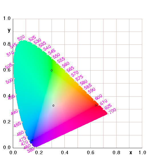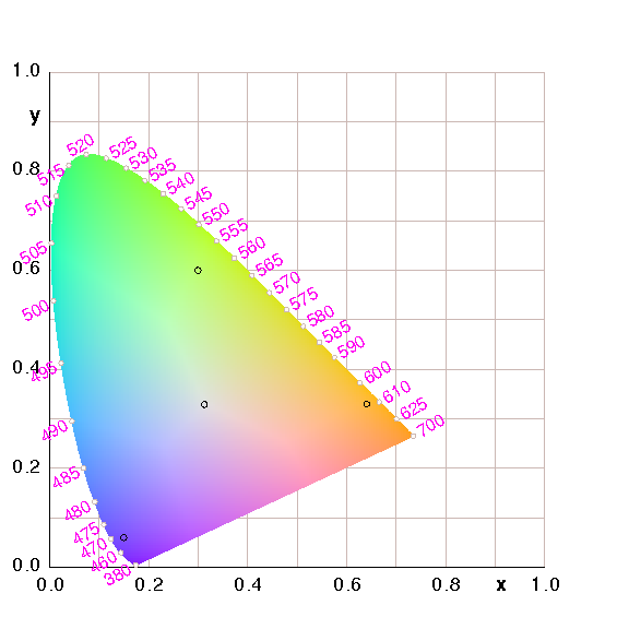
Figure 1: CIE Chromaticity Diagram for sRGB
This document has a few simple goals:
Parts of this problem are intrinsically hard. For instance there are some colors that simply cannot be represented on an ordinary CRT, LCD, or printer. I have ideas for improved hardware to alleviate some of the intrinsic problems, but that is beyond the scope of the this note, and the non-intrinsic problems discussed here would still need to be addressed, so here goes:
The shocking thing is that even within the limitations of existing hardware, there are a lot of problems for which solutions are known, yet the proper techniques are not widely used. As a result, there is lots of unnecessary trouble. For example, suppose you scan a picture to create a .jpg on your computer and look at it with an ordinary browser. In all probability it won’t look right. You have no way of knowing whether the file is messed up or whether your display is messed up. Or both.
Many files that look OK on a Macintosh look icky on a PC and vice versa. Many files that look OK on a CRT look icky on an LCD and vice versa. It is important to realize that it is possible to do much, much better.
The solution that works – the only solution that works – revolves around device profiles, as discused in section 5.
One thing that makes profiling practical is that each system only needs to know the profiles for its own input and output devices. Nobody needs to know much about the profile for anybody else’s devices.
This makes life simple: you just adjust your images until they look “right” on your display. Then (using your profile) you convert them to a portable device-independent format (as discussed below). Then you know you are publishing the right thing.
Your friends receive the device-independent representation and (using their profiles) the right colors will appear on their machines, or at least the most-nearly-right colors.
What you must not do is assume that your uncalibrated display is just like everybody else’s uncalibrated displays. There is a huge variation in displays, and it would be unwise (not to mention physically impossible) to make them all exhibit the same quirks. If you edit the picture so it looks good on your display, it will look icky on other displays.
Each of the following categories has its own quirks, so there will never be a “natural” or universally-correct match between any pair of them: CRT displays, LCD displays, printers, scanners, and cameras. Even within a category, there can be significant variation.
Calibrating a camera is harder than calibrating a scanner, because the camera is at the mercy of the ambient illumination. That means the calibration will change from scene to scene. You can pretty much plan on tweaking things by hand if you want them to come out right. Shoot a calibration target whenever you can. For a scanner, it probably suffices to calibrate it just once, since it provides its own illumination. The worst case is when you’re scanning photographic negatives; then you get all the uncertainties and nonidealities of the illuminant, the film physics, the development process, and the scanner – all at once.
We shall see that it is relatively easy for a computer program to correctly model the mixing of colored lights.
It is exceedingly hard to model the mixing of colored paints or inks. It is also exceedingly hard to model the effect of arbitrary illuminants on arbitrary colored objects. These are far beyond the scope of the present discussion.
A time-honored language for discussing color is the the tristimulus system from CIE (reference 1). This is also known as the XYZ system. Any pixel can be represented by three numbers [X, Y, Z]†, where X represents stimulus in the red channel, Y represents stimulus in the green channel, and Z represents stimulus in the blue channel, as perceived by a well-defined “standard observer”.
(Here we are thinking of these vectors as column vectors. For typographic convenience we write a row vector [...] and take the transpose using the † operator.)
We can calculate the chromaticity vector in terms of the tristimulus vector according to the simple rule:
| [x, y, z]† := |
| (1) |
If we project [x, y, z]† onto the xy plane, we get the familiar chromaticity diagram shown in figure 1. The denominator on the RHS of equation 1 probably has some fancy official name, but I haven’t ascertained what it is. It is roughly related to, but not exactly equal to, the perceived total brightness.
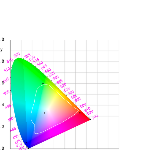
The horseshoe-shaped margin of the diagram represents the spectrally pure colors. Various points along the margin have been labeled with the corresponding wavelength in nanometers. The colors in the interior of the diagram are not spectrally pure, and neither are the colors along the lower-right edge (various shades of magenta and purple). These impure colors can be formed by mixing other colors.
Let’s take a closer look at the pure colors along the horseshoe-shaped margin of the diagram. For starters, consider the orangeish-yellow color of the sodium D line, which has a wavelength of 589 nm (reference 2). According to reference 3, that color is represented by the tristimulus value (1.110, 0.787, 0) or some multiple thereof (depending on overall brightness). Therefore, if I send you a file that calls for a color of (1.110, 0.787, 0) in this system, what you see on your display “should” match the color of a low-pressure sodium lamp. No real-world monitor can exactly match this color, but most “should” be able to approximate it reasonably closely. The system you are using probably won’t match it as closely as it should, which is why I’m writing this document.
The chromaticity of the sodium D line is (x, y) = (0.585, 0.415).
As a second example, the typical green laser pointer puts out a wavelength of 532 nm. That corresponds to an XYZ vector of (0.18914, 0.88496, 0.03694) or some multiple thereof. That corresponds to an xy (chromaticity) vector of of (0.1702, 0.7965). The key idea here is that the laser has a well-defined color and that color is unambiguously represented in the tristimulus representation. (Whether or not your monitor can represent this color is a separate question.)
In fact, typical monitors cannot match the 523-nm color very closely at all. We hope they do the best they can.
One nice thing about the CIE system is that it is well connected to the immutable laws of physics. In particular, it models the mixing of colored lights. That is, if we combine two light-beams by shining them onto the same spot, the result is well described by adding the tristimulus vectors in XYZ space.
A corollary is that the chromaticity of the result will lie somewhere along the straight line in xy space (chromaticity space) joining the chromaticity vectors of the ingredients. (You generally don’t know where along that line in xy space, unless you have additional information about the luminance of the ingredients.)
Figure 1 is optimized for viewing on an sRGB monitor. In the middle of the diagram there is a triangular region with relatively higher brightness. The area within this region is “in gamut” on an sRGB monitor. That is, the colors in this region are the only colors that an sRGB monitor can produce. The corners of this triangle are marked by black circles. These are the location of the Red, Green, and Blue primary colors on an sRGB monitor. These points correspond to the reddest red, the greenest green, and the bluest blue that the monitor can produce.
Near the middle of the diagram is a fourth black circle. This indicates the white point. This is the color that an sRGB monitor is supposed to put out when it is trying to represent white.
The points outside the sRGB triangle are perfectly well specified by their location in this diagram. These are perfectly good colors, but they cannot be represented on an sRGB monitor.
Actually, in figure 1 there are two reasons why points outside the sRGB triangle are not correctly depicted, i.e. why the color in the diagram does not correspond to the color that belongs at that (x,y) point on the CIE chromaticity diagram.
To repeat, in most cases where you are displaying an image file on a real device, there are device-gamut restrictions and file-gamut restrictions. A large part of the purpose of this dicument is to explain how to lift the file-gamut restrictions.
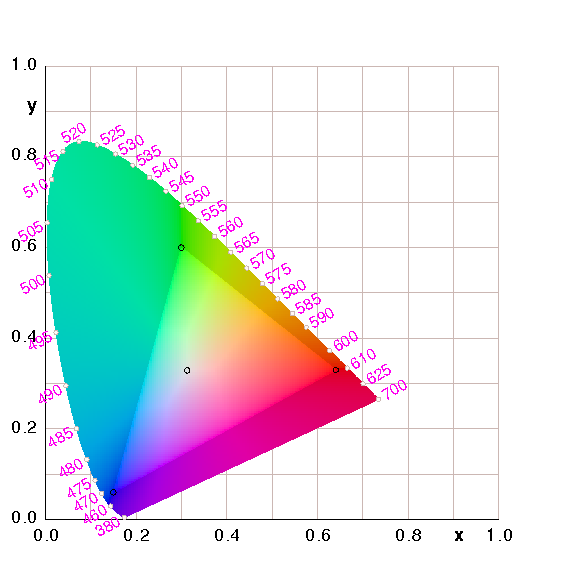
A couple of minor points can be made in connection with figure 2. This is the same as figure 1 except that I did not dim the colors that are outside the sRGB gamut.
The point we are emphasizing here is that the dimming used in figure 1 did not cause any of the limitations we are discussing here. Every point that is out-of-gamut in figure 2 is out-of-gamut in figure 1 and vice versa. The gamut boundary is just a little harder to perceive in figure 2, that’s all. (Calling attention to a problem is not the same as causing a problem!) This should have been obvious from the fact that these are chromaticity diagrams, and chromaticity (by definition) doesn’t encode any information about brightness, so changing the brightness cannot possibly affect the chromaticity.
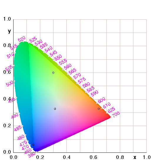
It may be useful to compare figure 3 with figure 4. If they look the same, there’s a problem.
|

| |
| Figure 3: CIE Chromaticity Diagram with Correct Wide cHRM | Figure 4: CIE Chromaticity Diagram with Bogus cHRM | |
The pixels in the two figures are the same, and both should look right when interpreted according to a wRGB profile. The .png file for figure 3 contains a cHRM tag correctly specifying wRGB, while figure 4 contains a cHRM tag specifying a wildly different color space (namely sRGB). The only way the two figures could look remotely the same is if your system is ignoring the cHRM tags.
According to the familiar oxymoron, the nice thing about standards is that there are so many to choose from.
There are umpteen different color management schemes (see reference 4). Many of them are quite well thought out. Alas, some of the most widely used are the worst.
Any good color management scheme ought to provide a device-independent way of describing colors ... but there is also a need for device-dependent colors. Suppose I am using a particular piece of RGB hardware. I’m not trying to communicate with anybody or publish anything. If I’m running ghostscript, and I say
0 1 0 setrgbcolor
that means I want to turn on the green dot on the display and turn off the other dots. The result should be some sort of green, a hardware-dependent green, the greenest green the display is capable of. Similarly if I say
.5 .5 0 setrgbcolor
that means I want to turn on the red and green dots, each halfway. The result should be some shade of yellow. If I don’t like this shade, it’s up to me to send a different command to the hardware.
Asking whether device-dependent colors are good or bad is like asking whether motor oil is good or bad. It depends. A certain amount of motor oil in the crankcase is good. Motor oil in your soup is bad.
Device-dependent colors are appropriate, indeed necessary for sending to the device. This is, after all, where the rubber meets the road.
In contrast, device-dependent colors are inappropriate as a form of publication, communication, or storage, unless you are sure nobody will ever want to use it on hardware different from yours.
A lot of color managment schemes have been proposed, but there is only one that makes sense to me. It revolves around the use of device profiles and color space profiles (reference 5).
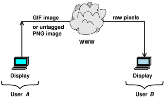
To prepare for the idea of profiling, consider the simple example shown in figure 5, which shows what happens if profiles are not used. User A prepares an image so that it looks good on his screen, and then sends the image in an untagged format to user B. The problem is that the image looks different on user B’s screen. That’s because user A and user B have inequivalent hardware, and the image was transmitted in a hardware-dependent format.
The PNG specification (to its credit) says that if the cHRM tag is absent from the image, the sematics of the image is hardware-dependent. GIF images are always hardware-dependent, and cannot be made hardware-independent.
In this example, user B is following an ultra-simple strategy, just taking bits off the web and throwing them onto his screen. Given what user A has done, user B is doing the best he can, indeed the only thing he can, unless he can somehow guess user A’s intentions and hardware configuration.
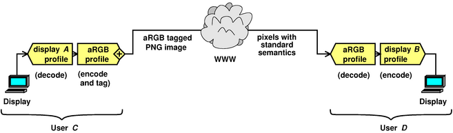
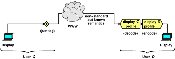
We can contrast this with the situation shown in figure 6, in which profiles are used to give a vastly better result. In particular, we see that the image on screen D is the same as the image on screen C.
The procedure here is as follows:
As a general rule, at this level of detail, every transformation uses two profiles back-to-back: one for decoding, and another for re-encoding. A profile is half of a transformation.
Note that the choice of format for pixels on the net is unimportant (over a wide but unlimited range). The encoding done by C is undone by D. All we require is that the encoding be lossless and invertible.
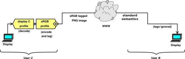
Yet another possibility is shown in figure 8. In this case, user C knows the profile of his display, but rather than transcoding anything, he simply puts onto the web the hardware dependent values that his display uses. The thing that makes this very different from figure 5 is that user C tags the outgoing image with the info about the color space of his display. Those tags are sufficient to allow astute user D to transcode from user C’s display color space to anything else, including D’s display color space.
Again this upholds the general rule that (at this level of detail) every transformation uses two profiles back-to-back: one for decoding, and another for re-encoding. A profile is half of a transformation.
There are also profiles that allow you to convert from one abstract color-space to another, for instance from XYZ to L*a*b*. It’s the same idea.
We can dream of a utopia in which images are stored in a completely abstract format that represents the author’s intentions, without regard for the limitations of any particular device. In the real world, this is arguably possible, but it is certainly not easy, and it is not widely done.
In practice, virtually all images one finds on the web are predicated on the assumption that they will be displayed on a screen, and probably something close to an sRGB screen. Little thought has gone into the possibility that the images will be printed on paper, or even displayed on a screen with capabilities much different from sRGB.
The problems are particularly acute for graphic artists who are preparing an image that will be used primarily for printing on paper ... yet they are using a computer screen to do the preparation. It is tricky to represent colors that are in-gamut for the printing process yet out-of-gamut for the preparation screen.
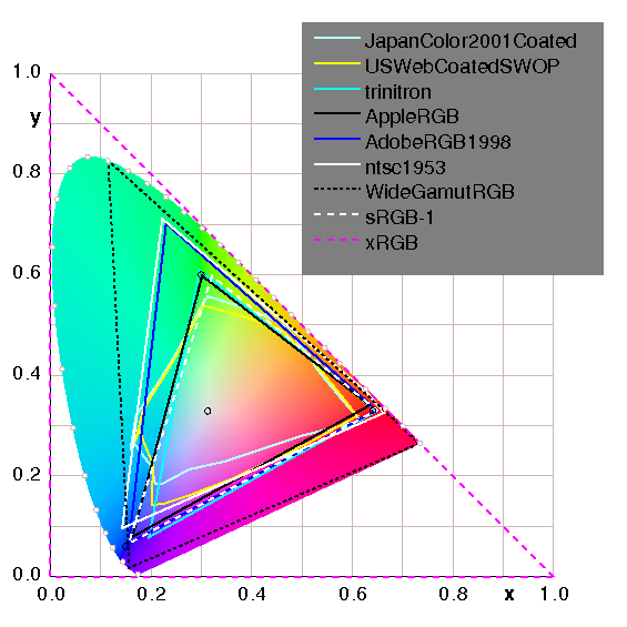
Please refer to figure 9. The idea for this comes from reference 6, which has several similar figures.
The purpose of the figure is to show the gamut of bright colors available in various profiles. Two of the outlines (JapanColor2001Coated USWebCoatedSWOP) apply to printers.1 Printers use ink, which multiplicatively removes photons from the image. (This stands in contrast to TVs and computer monitors which use lighted pixels and additively contribute photons to the image.) Therefore we are not surprised that the printer profiles have a very complicated non-triangular outline, and other complexities besides.
Next let’s look at the AppleRGB and sRGB-1 outlines.2 These are triangular, and very similar to each other. Their vertices almost (but not quite) coincide with the CCIR-709 primaries (represented by the black dots). This is discussed in section 11.1. The Trinitron outline is also similar, but its blue vertex is not quite as deeply saturated as the corresponding vertex of other profiles.
We now turn to the AdobeRGB1998 and ntsc1953 outlines. These are very similar to each other. They have a noticeably wider gamut than the five profiles mentioned in the previous two paragraphs. Indeed the AdobeRGB1998 profile is wide enough that it is almost a superset of the five aforementioned profiles.
The WideGamutRGB (aka wRGB) profile is even wider. It is a device-independent abstraction, not tied to any particular real-world hardware. (This is in contrast to all the profiles previously mentioned in this section, which model the properties of real hardware.)
Finally we come to the xRGB (“extended RGB”) outline, which encompasses the entire lower-left triangle in the diagram. Like the wRGB profile, it is a device-independent abstraction. It is wide enough to represent all possible colors ... and some impossible colors as well.
Note that any RGB model faces a tradeoff: If the primaries are real colors, then there will be some colors that cannot be represented in the model. Conversely, if the primaries are space widely enough to encompass all possible colors, they necessarily encompass some impossible colors as well.
Note that diagrams like figure 9 do not attempt to represent the entire gamut, just the bright colors in the gamut.
An ICC profile contains information about the entire gamut, and other information besides. It also describes the gamma curve, as discussed in section 9.
Here’s a challenge: Suppose you want to send your friends a really accurate version of the CIE chromaticity diagram – like figure 9 but with all the right colors in all the right places. Even after you figure out what goes where in theory, it’s not easy to find a file format in which you can store the answer, and not easy to find tools that will write such a file. When your friends receive such a file they won’t have an easy time rendering it.
To view or print a file containing device-independent colors, you need the device profile for your display or printer. (Actually the profile will depend not only on your printer but also on what type of paper you are using.) Profiles are typically stored in files with the .icc or .icm extension. The SCARSE project (reference 7) a library containing scores of profiles, plus tools for creating your own. Another large collection of profiles is available from reference 8.
Once you have profiles, you use various tools to apply them to your images. Reference 9, for example, provides a set of library routines you can link into programs, plus a simple command-line utility, tifficc, for applying profiles to .tiff files.
Adobe Illustrator and Photoshop have features for dealing with device-independent colors and device profiles, but not all the features work the way they should.
There are a number of color spaces that are device-independent and also complete (or overcomplete) in the sense that they can represent any perceivable color. The most widely-used examples are CIE XYZ and CIE L*a*b*.
There is also a recent creation called sRGB (standardized RGB; reference 10). It is device independent because it refers to standardized primary colors (defined in terms of CIE chromaticities) rather than whatever R, G, and B are implemented by the display you happen to be using today. Alas it is undercomplete; that is, it makes no provision for representing colors outside of the chromaticity triangle spanned by its chosen primaries. I’m not sure why anybody would want such a thing, when perfectly good overcomplete device-independent color spaces have been available all along.
There’s also "wide-gamut RGB" as discussed in section 12.
In principle, the original JPEG compression algorithm (reference 11) doesn’t care what color space you are using. But in practice when people speak of “JPEG” they mean the familiar .jpg file format, which is really JFIF. The JFIF standard (reference 12) specifies the ITU-601 color space (which is also called YCbCr, CCIR-601, PAL, and/or Yuv). This is in the same boat as sRGB: well-standardized primaries, but undercomplete. JFIF is the best available format for publishing natural scenes on the web. (For line drawings, as opposed to natural scenes, the JPEG compression scheme often introduces objectionable artifacts.)
The newer JPEG-2000 standard (reference 11) additionally includes support for the excellent CIE L*a*b* color space. So this opens a way of answering the challenge posed at the beginning of this section. You can get a free plugin (reference 13) to render .jp2 images in IE. There’s also a free plugin (reference 14) for Photoshop.
The .gif file format (reference 15) is out-of-date, and it wasn’t very good to begin with. It specifies neither standard primaries nor a standard gamma, so what you get depends on what brand of display the artist was using that day. (I hear rumors that the format can be extended to include color profile information, but I haven’t found any details on this. If such features exist they are exceedingly rarely used.) Just to rub salt in the wound, it uses a patented compression scheme, so there are no tools to write .gif files that are legal and free.
The .png file format (reference 16) is much better. You can put tags in the .png file that specify what colorspace the file is using (specified in absolute CIE terms). Similarly you can put in tags that specify the gamma (see section 9 for more on this). This works great.
(Of course with .png or any other system, you still need a calibrated display. Given a file that describes exactly what colors the artist intended, you can’t reliably display those colors unless you have calibrated your system.)
A .png file without a gamma tag and/or without a chroma tag means something very special. It does not mean to assume some canonical gamma or some canonical primary colors; instead it means to throw the bits onto the hardware, in a device dependent way, without applying any corrections. This is sometimes useful; remember what we said about motor oil. On the other hand, device dependence is rarely if ever appropriate for files that are to be published.
Windows-2000 has some hooks to support device profiles (right-click on the desktop background, device -> properties -> ...) but this may or may not be implemented, depending on what brand of display driver you’ve got. Furthermore, you may have to do some googling to find the .icm file for your display. Even then you’re not out of the woods, because microsoft browsers wantonly discard much of the color-space information in the .png file (reference 17).
Linux systems don’t have great support for device profiles, but you can at least calibrate the gamma, as discussed in section 9.
Alas only three formats (JPEG, .gif, and .png) are natively supported by present-day web browsers. So you really don’t have much choice:
The .pdf file format is a bit of a catch-all. It can handle device-dependent RGB and CMYK color spaces, as well as device-independent CCIR-601. Obviously if you want it to be portable you want to use the latter. This works reasonably well in typical cases, but the acrobat reader must be making some risky assumptions, because it has no provision for inputting the device profile of the display.
The .tiff file format (reference 18) is even more of a catch-all. It can handle device-dependent color spaces including RGB and CMYK, as well as device-independent color spaces such as CCIR-601 and CIE L*a*b*, plus other things (monochrome formats, transparency masks). (Note that what we call a color space is called a “photometric interpretation” in the .tiff header.) This flexibility makes it easy to write .tiff files – and difficult to read them in the general case.
Some features of the PostScript language antedate device profiles. The low-tech color operators in the language are setrgbcolor and setcmykcolor, which are unabashedly device-dependent; that is, they mean whatever your display or your printer takes them to mean. But ... things have gotten a lot better over the years. You can make device-independent images in PostScript (and/or PDF), as discussed in section 8. People are working on incorporating more general support for device profiles and device-independent color.
ImageMagick (reference 19) advertises that it can deal with device profiles, but these features are completely broken. Also, it appears to ignore the color-space declarations in .png files. Furthermore, it has not implemented any way to read .tiff files that use CIE L*a*b*, which leaves no way to read .tiff files that contain colors outside the restrictive RBG and CMYK gamuts. Maybe it is possible to get wide-gamut colors into ImageMagick by using the .pal (.uyvy) format – or maybe not; I am beginning to suspect that it uses some restrictive gamut internally and that choosing a new file format and/or improving the the I/O drivers would not be a full solution to the problem. Maybe the xRGB scheme (section 13) will allow ImageMagick to deal with wide gamuts.
The pngmeta -all command won’t disclose the gamma or chromaticity tags in a .png file, which is disappointing. You can use the identify -verbose command (part of the ImageMagick package) to display this information.
If you are using PostScript or PDF, and you want to maximize the quality and portability of your images, you should use the setcolorspace directive.
Doing so makes it entirely clear what you have chosen to use as the colorspace of your document, and tells the world how to convert your colorspace to the well-known device-independent CIE XYZ standard.
As I understand it, the conversion proceeds as follows:
| ABC | → | ABC* | → | LMN | → | LMN* | → | XYZ |
| | DecodeABC | | MatrixABC | | DecodeLMN | | MatrixLMN |
That is, the conversion involves three colorspaces (your document colorspace ABC, an intermediate colorspace LMN, and the final device-independent colorspace XYZ). MatrixABC and MatrixLMN are indeed matrices, so they can implement an arbitrary linear transformation. The Decode... functions can implement nonlinear transformations, and are typically used to apply “gamma” corrections, as discussed in section 9.
In many cases – notably whenever your document colorspace is some species of RGB – it suffices to set one of the Decode functions to be the identity transformation, and also to set one of the Matrix operators to be the identity matrix. In other cases, notably if your document colorspace is some species of CMYK, things are much, much more complicated.
Note: The matrices, as they are usually presented in PostScript files, have the appearance of the transpose of the matrices that appear in section 11. So beware. The program in appendix A knows to take the transpose when it should.
Things we can do: Life is easy if we just want to write PostScript programs in a highly-capable colorspace such as xRGB and then
Things we cannot do:
There are many things you would like to do in a linear RGB space. In particular, you might want to model the superposition of light sources, i.e. shining two primary light sources onto the same spot to produce a secondary color, such as RGB(1.0, 0, 0) plus RGB(0, 1.0, 0) makes RGB(1.0, 1.0, 0).
This is of great practical importance, because that’s how displays work. If you look closely, there are separate red, green, and blue pixels.
Things get trickier when we superpose two sources of the same color. In such a space we could add RGB(0.5, 0.5, 0.5) to itself to make RGB(1.0, 1.0, 1.0).
However, alas, digital image processing originated back when computer displays were CRTs (cathode ray tubes), which are highly nonlinear. Specifically, in terms of the color-codes presented to the monitor, RGB(0.5, 0.5, 0.5) was less than 1/4 as bright as RGB(1.0, 1.0, 1.0). We say such codes exist in a nonlinear RGB space.
The relationship between the code presented to the hardare and the resulting optical output is called the EOTF, ı.e. Electro-Optical Transfer Function.
Narrowly speaking the word gamma refers to a system or a subsystem where the output is related to the input by a power law, where the exponent is γ (the Greek letter gamma):
| O = Iγ (2) |
The CRT EOTF is very nearly a power law with a gamma of 2.2. As a result, loosely speaking, the word gamma is often used to refer to almost any EOTF, even when it’s not a power law. For instance many displays implement a “gamma ramp” which allows a multi-parameter EOTF, not described by a one-parameter power law. It really should be called an EOTF ramp.
In an ideal world, gamma would always equal unity, and we wouldn’t need to mention it. You would be able to use the postscript operator .5 .5 .5 setrgbcolor and get a 50% density gray color, and it would match what you would get from a 50% halftone.
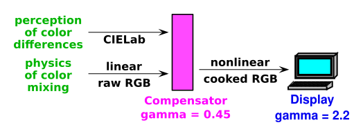
However, alas, we don’t live in an ideal world. It is important to correct for gamma at various points in the image-processing workflow. This is diagrammed in figure 10.
In particular, if you want to interpolate between colors, you should not do so in a cooked (nonlinear) color space such as sRGB. Instead you should uncook the color-codes, perform the interpolation in linear space, then re-cook as needed. Linear spaces include linear RGB (to model the mixing of lights) and CIELab (to model perceptible versus imperceptible changes in color). Perl code to perform the transformations is given in section B
There are 23 i.e. 8 colors for which none of this matters, namely black, red, green, blue, cyan, magenta, yellow, and white. That is, white, black, the three primaries, and the three secondaries. This is because both 0 and 1 are fixed points of the power law.
The situation was really ugly for a few years, but things have mostly settled down due to the emergence of the sRGB standard. Many monitors adhere implement sRGB. The standard specifies a particular EOTF which is nearly (albeit not exactly) the same as gamma = 2.2.
LCD screens, for which the physics is wildly different from CRTs, go out of their way to implement the nonlinear CRT-like sRGB profile. HTML standard says that the color-codes you put in your HTML style statements should be sRGB.
Even so, there remains some ambiguity. Sometimes when people say RGB they are referring to the linear RGB colorspace, and sometimes to the nonliear cooked RGB codes. For example, the X11 rgb.txt file predates the sRGB standard by many years. It defines gray50 as (127,127,127) on a scale of 0 to 255. Similarly it defines gray25 as (64,64,64). So that all seems nice and linear, i.e. not sRGB. On the other hand, the same file defines plain old gray as (190,190,190), which is suspiciously close to the code for 50% gray using the sRGB representation, i.e. (187,187,187). The bottom line is that I have no idea which entries in the RGB.txt file are meant to live in the raw color space or the cooked color space.
Typical uses mainly care about the color profile of their image, i.e. the color space in which their image lives. They want the overall system to faithfully render their image. In contrast, they don’t particularly care how many stage of processing are involved, or care about the EOTF of the individual stages, so long as the overall result is correct. (If you are designing one of the processing stages, then you care about a lot of things that ordinary users don’t, such as the stage-by-stage EOTFs.)
In figure 11, there are 12 squares. Within each square there is a diamond. Ideally, if you stand back and/or squint, the diamond should merge into the square background. All 12 of the diamonds should do this.
The three columns correspond to 25%, 50%, and 75% brightness, so they probe three points along the EOTF curve. They are implemented by turning entire pixels on and off, so they percentages live in a completely linear space. Meanwhile, the diamonds are colored using sRGB color codes. The point is, if your system adheres to the sRGB standard, the colors should match. You should not shrink the image too much, because you don’t want it to be degraded by the finite resolution of your screen. Insead, make the image reasonably large, then stand back and/or squint so that you cannot resolve the lines in the background squares.
You can also take a look at the smallish rectangle at the bottom of the image. It contains three diamond-shaped regions. The middle one is supposed to merge with the background. The other two, unlike all the others on this image, are not supposed to merge. One of them is 25% too bright, while the other is 25% too dark.
Remember: A decent characterization of your display requires knowing all the transfer-function information, plus the chromaticity of the three primaries and the white point (ie. RGBW). And as previously discussed, knowing RGBW is equivalent to knowing RGB including luminance information (not chromaticity).
Profiling a display from scratch requires a photometer – which you probably don’t have – to measure the chromaticities and brightness levels. You may be able to find on the web a suitable profile for your hardware; start by looking at reference 7 and reference 8.
In particular, users don’t have control over the chromaticity of the primaries on their display, so if you’ve got the transfer-function straightened out the only important variable that we haven’t dealt with is white-point chromaticity. This is usually not super-critical, because of the way the human brain perceives color: To a first approximation, the “whitest” thing in the field of view is perceived as white; this is a much better approximation than using some absolute context-free photometric notion of what “white” is.
In many cases of interest, color spaces are related to each other by fairly simple transformations. Often the transformation can be completely determined by specifying what happens to the primary colors, specifying what happens to the white point, and then invoking some normalization rules.
Let’s see how this works in the case of CCIR-709. It is related to (indeed defined in terms of) CIE. That is, the CIE chromaticity of the CCIR-709 primaries and white point are defined by
| (3) |
according to Table 0.2 in reference 10.
That’s all well and good, but it’s not the most convenient form for calculations. The numbers we are given specify only chromaticity directly; we will be able to figure out the intensity information, but it requires a bit of roundabout work.
It helps to separate the work into a linear piece and a nonlinear piece. So we introduce a third color space, the CIE (X, Y, Z) space. It is linearly related to CCIR-709, whereas the connection to chromaticity itself (x, y) is nonlinear.
By way of preliminaries, let’s do something that doesn’t quite work. Let’s try to write a matrix that connects the CCIR-709 primaries to the chromaticity vector:
| (4) |
This has got several related problems. First of all, if we treat this as a matrix and set (R G B) to (1 1 1) we get (x y z) values that don’t make any sense at all; they are not properly normalized. And even if we wave a magic wand and normalize them, we get a chromaticity vector that doesn’t match the stipulated white point. Thirdly, the matrix is not invertible, so we won’t be able to find the mapping in the other direction, from (x y z) to CCIR-709. But we should have known that in advance; (x y z) doesn’t encode any intensity information, so there was never any hope of finding the inverse mapping.
The last point is the key to making progress. Knowing the chromaticity of the R, G, and B sources is necessary but not sufficient, because it doesn’t specify the relative intensity of the sources. That’s why the definition (equation 3) includes additional information, namely the white point.
Let’s be clear about this: There are four nontrivial constraints that we need to satisfy (plus a fifth relatively trivial one):
So what we are looking for is a matrix that is related to the one in equation 4, but where each column has been multiplied by some scale factor. We find appropriate scale factors to make the white point come out right. A suitable result is:
| (5) |
which corresponds to equation 1.1 in reference 10.
This has none of the problems of the previous matrix. Multiplying this matrix against an RGB vector gives a nicely un-normalized [X, Y, Z]† vector; we can normalize the latter if we want, in the natural way:
| (6) |
As an exercise, you should confirm that if you multiply the matrix in
equation 5 by the RGB white vector [1, 1, 1]†, then
normalize, you do in fact get the desired chromaticity for the white
point as given in equation 3.
The matrix in equation 5 is nicely invertible; the inverse is:
| (7) |
Note that any multiple of these matrices would do just as well, because the CCIR-709 color space is specified by four chromaticities (the three primaries and the white point), so the overall brightness of the display is not specified. I have exercised this gauge freedom to make the middle row in equation 5 sum to unity, for reasons discussed in section 8. When you take arbitrariness of the normalization into account, there are only eight interesting numbers in this matrix. It is no coincidence that the original data (the four chromaticities in equation 3) also consisted of eight numbers.
To construct equation 5, starting from the givens in equation 3, we have to find scale factors for the red column and the green column. This involves two equations in two unknowns. The code to solve this and print out the transformation matrix presented in appendix A.
The sRGB color space is closely related to CCIR-709, but there are additional complexities. There are nonlinearities involved. For details, see reference 10 and look at equation 1.2 and the associated discussion of sR’G’B’.
You can play the same games with the ITU-601 color space, which is used in .jpg (JFIF) files and elsewhere.
But you have to be careful. There is a theoretical definition of the Yuv color space, but that’s not quite what people use in computer programs. To quote from libjpeg/jdcolor.c:
 * YCbCr is defined per CCIR-601-1, except that Cb and Cr are
 * normalized to the range 0..MAXJSAMPLE rather than -0.5 .. 0.5.
 * The conversion equations to be implemented are therefore
 *      R = Y                + 1.40200 * Cr
 *      G = Y - 0.34414 * Cb - 0.71414 * Cr
 *      B = Y + 1.77200 * Cb
 * where Cb and Cr represent the incoming values less CENTERJSAMPLE.
 * (These numbers are derived from TIFF 6.0 section 21, dated 3-June-92.)
What that means is that the Cb (u) channel and the Cr (v) channel have been shifted so that neutral gray is at (u,v) = (0.5, 0.5) (rather than zero) and rescaled so that the red primary has v=1.0 and the blue primary has u=1.0. Then eacy of the numbers (Y, u, and v) is converted to a fixed-point representation, by multiplying by the largest representable integer (MAXJSAMPLE).
In my humble opinion, this wasn’t the wisest possible rescaling. Whereas the original CCIR-601-1 specification was overcomplete in principle, the rescaling leaves us with a colorspace that is undercomplete in practice. It can represent all the colors inside the triangle (in chromaticity space) spanned by its primaries, and a few nearby colors, but there are lots of perceivable colors that it cannot represent. If they had provided a little more “leverage” in the u and v channels, they could have covered the entire range of perceivable colors. Apparently they weren’t thinking outside the box that day.
Similar remarks apply to sRGB or any other undercomplete color space: It could become complete if you could find a way to let the components vary over a wider range, for instance letting the R component be less than zero or greater than one. See section 13.
Anyway, the defining points for ITU-601 are:
| (8) |
which differs from CCIR-709 in only one component, namely the x component of the green primary.
Using the methods of section 11.1 we can figure out the relative intensity of the three primaries, so as to produce the stipulated white point. We obtain the following matrix, which converts an RGB point (using the ITU 610 primaries) to to absolute, physically-defined CIE colors:
| (9) |
And we will also need the inverse of that:
| (10) |
But there’s more to ITU-601 than just the choice of primaries; there is also a coordinate transformation to Yuv coordinates. The matrix for that is:
| (11) |
And the inverse transformation is:
| (12) |
Suppose somebody defines a fairly-wide-gamut color space using primaries on the boundary of the perceivable colors. You could in principle build a display that implements these primaries, using lasers or some such... but more typically this color space is just an abstraction. Real-world hardware will use primaries that lie in the interior of the wide-gamut color space. This is good, because it means that files using the wide-gamut representation will be portable to different types of hardware.
In figure 12, the region in xy space within the large triangle of bright colors defines the gamut for something called "the" Wide RGB color space. The darker colors outside this triangle are not even represented correctly in the file, so it doesn’t even matter whether your display can handle them; they are guaranteed wrong. Within the triangle, there are various possibilities:
The wide RGB primaries are:
| (13) |
which leads to the transformation matrix:
| (14) |
And the inverse thereof:
| (15) |
The CMYK gamut in figure 12 is not a guess or an opinion; it is real data. I got it by writing a program to map out the color-management profile for a particular printer/paper combination. I don’t know how to explain the exact shape of the gamut; I’m just presenting the data as it came to me in the .icm file. The physics of mixing inks (CMYK) is much more complicated than the physics of superposing light sources (RGB).
This CMYK data is device dependent; your printer/paper combination presumably has a different gamut. But I figured showing you some device-dependent data would be better than no data at all.
As you can see in figure 9, there are many different ways of choosing three primary colors. But no matter which of those you choose, there will still be lots of out-of-gamut colors. (You can do lots better if you use more than three primary colors.)
But if we think outside the box a little bit, we can invent a set of primaries that span all perceivable colors. The following will do the job: We choose the following primaries, and once again use the D65 white point:
| (16) |
I call this the xRGB color space – extended RGB. Its gamut is the whole triangle below the y=1−x diagonal in figure 13.
Again we use the white-point information to derive the properly un-normalized transformation matrix, to wit:
| (17) |
The inverse transformation is given by:
| (18) |
To see how this works, consider spectrally-pure light of 700 nanometer wavelength. It has chromaticity xy = [0.7347, 0.2653]†. As a exercise, you can check that this corresponds to an xRGB vector of [1.0, 0.3432, 0]†, which tells us that this point lies on the straight line between the red primary (xy = [1, 0]†) and the green primary (xy = [0, 1]†) with no significant admixture of blue ... as it should. Similarly, for 505 nm light, the chromaticity is [0.0039, 0.6548]†, and the corresponding xRGB vector is [0.006, 1.0, 0.4786]†, which lies very close to the line between the green primary and the blue primary, with very little admixture of red ... as it should.
Figure 13 was made using these techniques.
The fact remains that even though the file encodes all the right colors, your hardware cannot possibly reproduce them all Note the contrast:
This is where the hardware issues meet the software issues. If we want to display more-beautiful images, we need more-capable hardware and we need file-formats that can invoke the new capabilities. The file-formats, which are the topic of this document, ought to come first.
It is possible (indeed, alas, likely) that figure 13 will look completely wrong on your system; even the subset of the diagram that lies within the gamut of your system will be off-color. The problem is that some software performs unduly intolerant checks on the chroma tags in .png files. They may well reject the tags in this figure, and proceed to throw the bits onto the display in the default (hardware-dependent) way, which is going to be quite a mismatch.
This was a problem in pre-2006 versions of libpng. The code at libpng.org has been fixed, but the fixes have been slow to propagate into the widely-used distributions.
The right thing to do is to (a) get the up-to-date code, (b) recompile the dynamic libraries, and (c) rebuild any applications that have static copies of the libraries. Alas that’s more work than most people want to do.
This image is a bit ahead of its time. I have not yet found any software that will display it correctly. Mozilla won’t. Konqueror won’t. MSIE won’t. Gimp won’t. Opera doesn’t even handle gamma tags, let alone chromaticity. ImageMagick never applies chromaticity information. This is after removing the bounds-checking from all my libpng libraries.
In general:
As of the moment, when publishing images on the web:
If your audience is mostly PC users, try to arrange things so that you can declare gamma=.45 in your .png files. The compensates for the gamma=2.2 that is fairly typical of PC-type monitors, and maximizes the chance that things will look OK if the PC software ignores the gAMA information. Meanwhile, if your audience is mostly Mac users, try to arrange for gamma=0.56=(1/1.8). Similarly, if your audience is mostly SGI users, aim even lower, namely gamma=0.7=(1/1.43).
When doing calculations, don’t be in a big hurry to collapse the three-dimensional tristimulus representation (X, Y, Z) into the two-dimensional chromaticity representation (x,y). That latter is great for visualizing certain properties of the color, but it loses intensity information. The Yxy representation keeps the intensity information, and is nice for thinking about color, but it is nonlinear and not maximally convenient for calculations, so keep those conversion subroutines handy.
This is a program in the language of scilab, which I chose because of its excellent vector- and matrix-handling abilities. (It is very similar to MatLab.) The scilab system runs on windows as well as Unix, and can be downloaded for free from www.scilab.org.
Reference 21 contains some code to calculate transformation matrices, but it is much less numerically-stable than my code, and in particular it barfs on the xRGB → XYZ transformation.
//////////////
//
//  exec "tmatrix.sci";
//
// Solve for the transformation matrix
// (chromaticity as a function of document-space color)
// given the chromaticity of the document's
// white, red, green, and blue points.

// Calculate the transformation matrix
//  that goes from document-space to CIE-XYZ.
// Call here with four chromaticity vectors:
// white, red, green, blue

function lmn=tmatrix(w, r, g, b)
// Here dr, dg, and db are vectors in the xy plane, i.e.
// vectors from the white point to each primary:
  dr = r-w;
  dg = g-w;
  db = b-w;

// Take the ratio of wedge products:
// Logically wedge(db,dr) would be multiplied
// into the middle column, but we divide
// it out of the whole matrix to achieve
// conventional normalization.
  kr = wedge(dg,db);
  kg = wedge(db,dr);
  kb = wedge(dr,dg);
// Add a regularizer term to protect against singular cHRM
// data, i.e. "zero area" situations
// i.e. where the primaries are collinear or coincident:
  if kr == 0 then kr = 1e-6; end;
  if kg == 0 then kg = 1e-6; end;
  if kb == 0 then kb = 1e-6; end;

// coerce them to columns (not rows) to defend
// against a common user error:
  rr = column(r);
  gg = column(g);
  bb = column(b);

// generate the third component:
  rr(3) = 1 - rr(1) - rr(2);
  gg(3) = 1 - gg(1) - gg(2);
  bb(3) = 1 - bb(1) - bb(2);

// make the matrix:
  lmn = [ rr*kr, gg*kg, bb*kb];

// normalize:
  lmn = lmn / sum(lmn(2,:));

endfunction


function cv = column(v)
  s = size(v);
  if s(2) == 1 then cv = v;
  elseif s(1) == 1 then cv = v';
  else error("Neither row nor column");
  end

endfunction

function xy=chromaticity(XYZ)
  denom = sum(XYZ(:));
  printf("%g %g %g\n", XYZ(1), XYZ(3), denom);
  xy(1) = XYZ(1)/denom;
  xy(2) = XYZ(2)/denom;
endfunction

// Returns the wedge product of two vectors in D=2.
// You can consider the result either an area or a pseudoscalar.
function ps=wedge(V, W)
  ps = V(1)*W(2) - V(2)*W(1);
endfunction

function latexprint(lbl, mmm)
  for jj=1:3
    printf("%6s & %8.4f & %8.4f & %8.4f  \\\\\n", lbl(jj), mmm(jj,:));
  end
endfunction

function print2(fwd)

  latexprint(["X:", "Y:", "Z:"], fwd);
  printf("\n");

  if det(fwd) == 0 then
    printf("Singular!\n");
  else
    rev = inv(fwd);  // matrix inverse
    latexprint(["R:", "G:", "B:"], rev);
  end;

endfunction

function xyz = chty(lmn, rgb)
  XYZ = lmn * rgb;
  xyz = XYZ / sum(XYZ);
endfunction

function [w, r, g, b]= parse(sss)

  [ wx wy rx ry gx gy bx by ] = sscanf(sss, ...
   "%g %g %g %g %g %g %g %g");

  w = [wx, wy]';
  r = [rx, ry]';
  g = [gx, gy]';
  b = [bx, by]';

endfunction

// Scilab's list-handling powers are not sufficient to
// allow us to write tmatrix(parse(adobe)) directly,
// so we brute-force it:
function mmm = tmatrixp(sss)
  [w, r, g, b] = parse(sss);
  mmm = tmatrix(w, r, g, b);
endfunction

function adoprint(mmm)
  wp = mmm * [1, 1, 1]';
  printf("%s\n%s\n%s\n%s\n%s\n%s\n%s\n%s\n",...
    "[",...
    "  /CIEBasedABC",...
    "  3 dict dup dup dup",...
    "  /DecodeLMN [",...
    "    {gamma exp} bind",...
    "    {gamma exp} bind",...
    "    {gamma exp} bind] put",...
    "  /MatrixLMN [");
  mmmt = mmm';
  for jj=1:3
    printf("  %8.4f %8.4f %8.4f\n", mmmt(jj,:));
  end
  printf("%s\n%s\n",...
  "  ] put",...
  "  /WhitePoint [");
  wpt = wp';
  printf("  %8.4f %8.4f %8.4f\n", wpt)
  printf("%s\n%s\n",...
  "  ] put",...
  "] setcolorspace");

  printf("\n/cspace-inv { %% Inverse mapping:\n");
  www = inv(mmm);
  lbl = ["R", "G", "B"];
  for jj=1:3
    printf("  /%s  %8.4f x mul  %8.4f y mul add  %8.4f z mul add  def\n",...
      lbl(jj), www(jj,:));
  end
  printf("} def\n");


endfunction


/////////
// usage: map1(wide)
//
function map1(gmt)
  mmm = tmatrixp(gmt);
  www = inv(mmm);
  for jj = 0 : 10
    kk = exp(jj-5);
    rgb = [ 0, 1, kk]';
    xyz = mmm * rgb;
    xyzn = xyz / xyz(2);
//    xyzn /=  3.564;  // for wide
//    xyzn /= 3.456;  // for sRGB
    xyzn = xyzn / 13;  // for sRGB, blue only
    rgbn = www * xyzn;
    printf("%7.3f %7.3f %7.3f    %7.3f %7.3f %7.3f\n", xyzn', rgbn');


//    printf("%7.2g %7.2g %7.2g    %7.2g %7.2g %7.2g\n", rgb', xyz');
//    printf("%7.2g %7.2g %7.2g    %7.2g %7.2g %7.2g\n", xyz', xyzn');

  end

endfunction

//////////////////////////////////////////////////////////////////////
// main program:

// they must be given in order: w r g b
// (which is the way the ppm2png -chroma arguments work),  e.g.
sRGB=   "0.312713 0.329016  0.6400 0.3300  0.3000 0.6000  0.1500 0.0600";
itu601= "0.312713 0.329016  0.6400 0.3300  0.2900 0.6000  0.1500 0.0600";
wide=   "0.3457   0.3585    0.7347 0.2653  0.1152 0.8264  0.1566 0.0176";
xRGB=   "0.312713 0.329016  1.0    0.0     0.0    1.0     0.0    0.0";
// From page 7 of 5122.MatchRGB.pdf :
adobe=  "0.3127   0.3290    0.6250 0.3400  0.2800 0.5950  0.1550 0.0700";
weird=  "0.3127   0.3127    0      0.3127  0      0.3127  0      0.3127";
play=   "0        0.3127    0      0.3127  0      0.3127  0      0.3127";

  white = [1, 1, 1]';
  red = [1, 0, 0]';
  green = [0, 1, 0]';
  blue = [0, 0, 1]';


// A common useful idiom:
//
//++   print2(tmatrixp(adobe));
// ..or..
//++   print2(tmatrixp(play));

// compare the given chromaticity with the calculated one:
//++  r, chty(fwd, red)

// The example from tn5122:
  ado = [0.4497 0.2446 0.0252 ;
  0.3163 0.6720 0.1412 ;
  0.1845 0.0833 0.9227];

// A nice check is to subtract ado-mine :
  mine = tmatrixp(adobe)';

// Another nice check:
//++ adoprint(tmatrixp(adobe))
// and compare that with the numbers on page 8 of tn5122
my $phi = 12.9232102; ## inverse slope in the linear region
my $crossover = 0.0392857;
my $Gamma = 2.4;                # exact
my $affine = 0.055;             # exact

sub eotf {
  my ($x) = @_;
  return $x/$phi if $x <= $crossover;
  return (($x + $affine) / (1 + $affine))**$Gamma;
}

# y = x/phi
# x = y * phi
# y**invg * (1+affine)  - affine = x

sub inveotf {
  my ($y) = @_;
  return $y*$phi if $y <= $crossover/$phi;
  return $y**(1/$Gamma) * (1 + $affine) - $affine;
}