|
| |
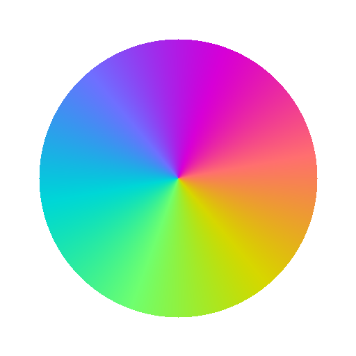
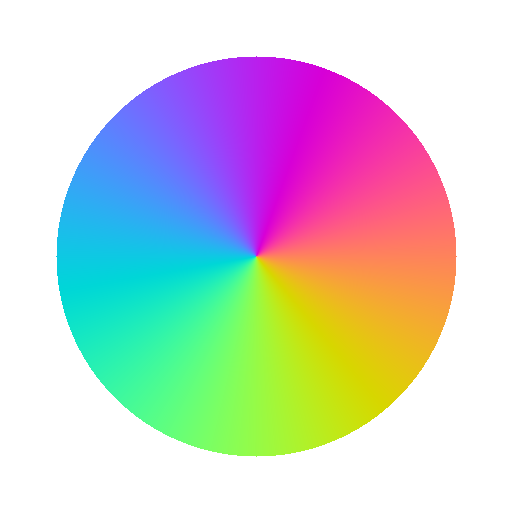
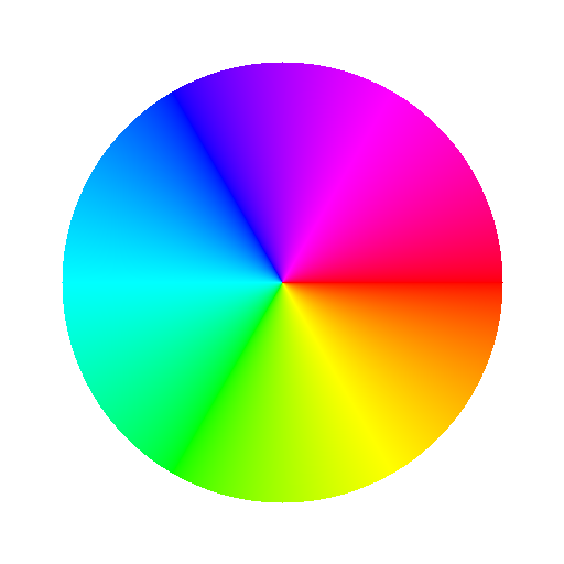
| Figure 1: Disk with Rays | Figure 2: Disk with No Rays | |
Let’s consider the disk-shaped images shown in figure 1 and figure 2. Presumably you can see that the two figures are not quite the same. In particular, in figure 1, you can see six so-called bright rays. These are more prominent near the center, and they are more prominent if you view the figure from a greater distance.
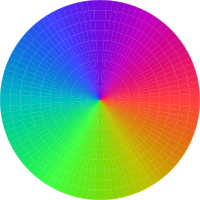
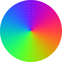
In case you are wondering whether you are seeing rays (or lack thereof) due to some peculiarity in your display hardware, figure 3 and figure 4 show the same data, just rotated 10 degrees. The pattern we wish to discuss should be rotated; any display artifacts should remain unrotated.
The bright rays are an optical illusion. Also, the bright dot in the middle of both disks is an optical illusion. Let us try to understand this a little bit.
Both disks were constructed in such a way that the brightness is very nearly constant across the disk. You can confirm this using a photometer, or by measuring the RGB values of the individual pixels. Figure 5 shows the innermost pixels of figure 2, enlarged by a factor of 2000%, demonstrating that there is no “dot” at the center of the disk.
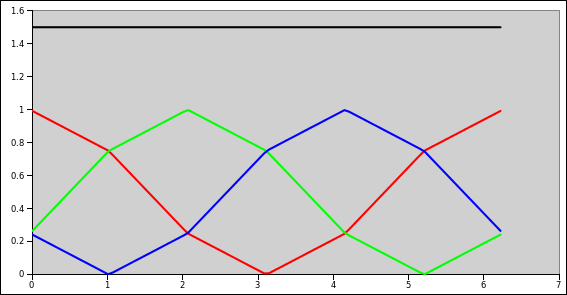
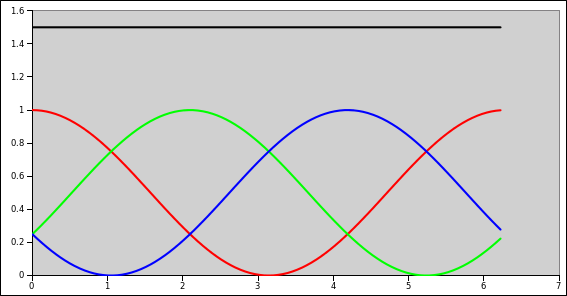
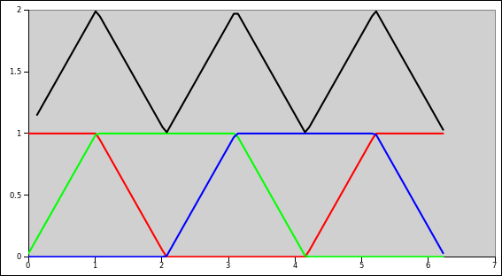
We can get a idea of what is going on by reference to figure 6 and figure 7. These figures plot the red, green, and blue pixel values as a function of azimuth around the disk. You can see that the six so-called bright rays correspond to places where there is a spike in the second derivative of hue with respect to position. That is to say, the rays are observed where there is a change in the rate-of-change of hue with respect to position. In non-technical terms, we can say that a crimp in the hue is perceived as brightness ... even when there is no significant change in the photometric brightness.
This demonstrates that perceived brightness is not the same as photometric brightness. Evidently a crimp in the hue is perceived as a bright ray-like feature, even when there is no such feature in the photometric brightness.
This has probably been known to experts in the field for several decades, if not centuries. However, it came as a surprise to me.
In particular, I thought there was a rule of thumb associated with NTSC YUV color encoding, to the effect that the eye is sensitive to sharp changes in luminance, but not nearly so sensitive to changes in chrominance. I’m not terribly surprised to find that the eye is sensitive to the Lapacian of hue, and/or the Laplacian of the individual color components ... but I am surprised that a crimp in the hue is perceived as brightness ... as opposed to some other percept.
Similarly, there are lots of color spaces (YUV, L*a*b*, HSV, et cetera), where there is an attempt to represent brightness or lightness as being orthogonal to hue. However, the examples shown here demonstrate that perceived brightness is not independent of hue ... quite noticeably not.
I am further surprised that this result is inconsistent with the standard drafting practice of emphasizing the edges on a colored object by drawing a black line. Maybe a bright-colored line would be better.
There is a vast literature on the “receptive fields” of neurons, including second-derivative detectors, but the landmark papers (reference 1 and reference 2) emphasized black-and-white vision, and all of my experience in image processing has dealt with black-and-white images. Also I have read some papers that indicated that the human vision system used an “opponent-color” representation, which would seem to imply that hue is handled differently from brightness ... but we now see that there is more to the story.
If anybody knows of a reference where this illusion is discussed, and/or knows of a name for this illusion, please let me know.
The fact that the rays look different depending on how close you are to the diagram tells us something about the size of the receptive field of the neurons involved.
Here’s the closest I can come to understanding this: If we process red, green, and blue separately, and run each of them through a filter that takes the magnitude of the second derivative, a crimp in the red channel will be perceived as “more red” and similarly for blue and green. So, if I am interpreting this correctly, it means that – at least at some stage in the processing – a simple R, G, and B representation is being used (as opposed to any sort of opponent-color representation, or anything fancy like YUV, L*a*b*, or HSV).
That’s interesting, because representations such as L*a*b* are touted as being “perceptual” representations. They are good for predicting some important perceptions, such as metamerisms. However, not all perceptions play by the same rules. Evidently different representations are used in different parts of the vision system.
In figure 6 and figure 7, the black line is the total of R+G+B, which you can see is constant. Now R+G+B is not quite the same as brightness, but it is close, and in any case it is clear that the photometric brightness is slowly changing as a function of position.
You may be wondering why anybody would be tempted to use the functions shown in figure 6. Well, those functions can be considered a modification of the standard RGB ↔ HSV conversion functions, as shown in figure 9. Note that the HSV representation (hue, saturation, and value) is widely used in “office computing” applications including spreadsheets and word processors. It is even used in books on color intended for use by artists. It is not, however, very sophisticated. Suffice it to say, if you want to make a nice-looking color wheel, just going around the hue circle and doing an HSV → RGB conversion is not going to look nice. There will be wild variations in photometric brightness as you go around the circle ... as well as a severe case of the “bright rays” illusion ... as you can see in figure 8.