Figure 1: Density Altitude versus Temperature
The “standard” atmosphere is a model. It is artificial, but it agrees reasonably well, on average, with the real atmosphere on a cool day in temperate regions.
This is sometimes called the “International Standard Atmosphere”, and I will call it the ISA model for short.
The ISA model consists of seven layers, labeled zero through six inclusive. The properties given in the following table.
| Layer | Height | Pressure | Density | Temperature | Lapse | Name | |||||
| (m) | (ft) | (Pa) | (inHg) | (kg/m3) | (K) | (C) | (K/m) | (K/ft) | |||
| 0 | 0 | 101325 | 29.92126 | 1.224999 | 288.15 | 15.00 | Sea Level | ||||
| 0 | ⋮ | ⋮ | ⋮ | ⋮ | ⋮ | ⋮ | ⋮ | 0.0065 | 0.0019812 | Troposphere | |
| 11,000 | 36,089 | 22632.1 | 6.683246 | 0.363918 | 216.65 | -56.50 | Tropopause | ||||
| 1 | ⋮ | ⋮ | ⋮ | ⋮ | ⋮ | ⋮ | ⋮ | 0 | 0 | Stratosphere(a) | |
| 20,000 | 65,616 | 5474.89 | 1.616734 | 0.088035 | 216.65 | -56.50 | |||||
| 2 | ⋮ | ⋮ | ⋮ | ⋮ | ⋮ | ⋮ | ⋮ | -0.0010 | -0.0003048 | Stratosphere(b) | |
| 32,000 | 104,986 | 868.019 | 0.256326 | 0.013225 | 228.65 | -44.50 | |||||
| 3 | ⋮ | ⋮ | ⋮ | ⋮ | ⋮ | ⋮ | ⋮ | -0.0028 | -0.0008534 | Stratosphere(c) | |
| 47,000 | 154,199 | 110.906 | 0.0327506 | 0.001428 | 270.65 | -2.50 | Stratopause | ||||
| 4 | ⋮ | ⋮ | ⋮ | ⋮ | ⋮ | ⋮ | ⋮ | 0 | 0 | Mesosphere(a) | |
| 51,000 | 167,322 | 66.9389 | 0.0197670 | 0.000862 | 270.65 | -2.50 | |||||
| 5 | ⋮ | ⋮ | ⋮ | ⋮ | ⋮ | ⋮ | ⋮ | 0.0028 | 0.0008534 | Mesosphere(b) | |
| 71,000 | 232,939 | 3.95642 | 0.00116833 | 0.000064 | 214.65 | -58.50 | |||||
| 6 | ⋮ | ⋮ | ⋮ | ⋮ | ⋮ | ⋮ | ⋮ | 0.0020 | 0.0006096 | Mesosphere(c) | |
| 80,000 | 262,467 | 0.88628 | 0.000261718 | 0.000016 | 196.65 | -76.50 | Mesopause | ||||
The staggered rows in the table are meant to indicate the layers and the boundaries between layers; for instance, layer #1 extends from 11,000 meters to 20,000 meters, and within this layer the lapse rate is zero. At the tropopause, i.e. the boundary between layer #0 and layer #1, the pressure is 22632.1 pascals. You can compare this table with the one in reference 1.
Some discussion of the range of validity of this table, and extensions to the range, can be found in section 2.
Generally speaking, we are interested in all of the following:
The standard model of the atmosphere makes assumptions about the last two (temperature and chemical composition). It also makes assumptions about the sea-level values for the other two (pressure and density). These assumptions are reasonably close to reality, but not exact.
Given those assumptions, the pressure and temperature at other altitudes are determined by the laws of physics.
So, to model the atmosphere we need the following:
All the other numbers in the table can be calculated using the quantities listed above.
So, without further ado, let discuss how to compute the properties that need to be computed. We start from layer #0 and work our way up. We will need the force-balance equation (equation 1) and the ideal gas law (equation 2).
We can view the force balance in either of two ways. The first view starts from the observation that at any height h, the pressure is equal to the weight (per unit area) of the air column above h. This makes sense in terms of conservation of momentum (aka force balance), since something has to support the weight of the air column.
Pressure is defined as force per unit area, and in this case the force is the weight of the air column.
The second view takes a more local approach, treating the air column as many parcels of air, stacked up like pancakes. Then dP is the increment of pressure contributed by a single parcel dh thick. You can see that ρdh is the mass per unit area of the parcel, ρgdh is the corresponding weight, i.e. the force of gravity. Putting this all together gives us the force-balance equation:
| (1) |
The minus sign reflects the fact that pressure decreases as height increases.
You can easily show that the two views do in fact represent the same physics. Integrate equation 1 from h to infinity, and as a boundary condition use the fact that the pressure is zero in outer space.
Meanwhile, the ideal gas law is:
| (2) |
where we are using the following symbols:
| (3) |
So far, we have used only the general laws of physics. We now make some assumptions that are specific to the standard atmosphere. Here are the assumptions, and some comments about them:
| We assume that the density is low enough that the idea gas law is valid to high precision. | This is a very well-founded assumption. |
| We postulate that the molar mass in the standard atmosphere is constant, namely mM = 28.9644 grams per mole. | The molar mass of the real atmosphere varies according to humidity and other factors, but still this value of mM remains a good approximation. |
| We postulate that in the standard atmosphere, the pressure equals 101325 pascals when the height equals zero. | The real atmosphere often deviates significantly from this, so it will be necessary to apply an offset – the Kollsman offset – to the standard atmosphere before using it for practical applications such as altimetry. This is what ordinary altimeters do, as discussed in detail in section 3. |
| Last but not least, we postulate that the lapse rate in the standard atmosphere is as specified in the table. | In the real atmosphere, there can be a significantly non-standard lapse rate, often associated with a non-standard temperature. In some situations, this can be handled to zeroth order using a Kollsman offset as previously mentioned ... but in other situations the zeroth-order (Kollsman) approximation be dangerously misleading, as discussed in section 4. |
The lapse is expressed by the following equation:
| (4) |
where for any layer, λ is the lapse rate for that layer. Equation 4 can be immediately integrated to give a widely useful result:
| (5) |
where, for any given layer:
| (6) |
for some “baseline” point within the layer, as indicated by the subscript “b”. (Very commonly the baseline is taken to be the bottom of the layer, but actually you are free to choose any point within the layer where the temperature and pressure are known, as discussed in section 2.)
In the troposphere, the temperature gradient dP/dh is negative, and the lapse rate λ is a positive number, namely λ = 0.0019812 C/ft. In other words, 2 degrees C per thousand feet.
Starting from equation 1 and plugging in equation 2 and equation 4, we arrive at:
| (7) |
which is easily integrated. For any layer in which the lapse rate is nonzero, the main result is:
| (8) |
where in the exponent we have introduced the dimensionless constant N, defined as:
| (9) |
In the troposphere, N is a positive number, N ≈ 0.1902632, so 1/N ≈ 5.25588.
You can verify the correctness of equation 8 by differentiating both sides with respect to h and comparing it to equation 7.
In the special case where the lapse rate is zero, the main result reduces to:
| (10) |
as you can verify by direct integration of equation 7, or by differentiating both sides of equation 10 with respect to h, or by taking equation 8 in the limit as λ goes to zero, with due regard to the λ-dependence of N.
Out of curiosity, we can see what would happen if the bottom layer of the atmosphere were isothermal. Using the ISA sea-level temperature, we would have:
| (11) |
We can solve equation 8 to give height in the standard atmosphere (i.e. pressure altitude) as a function of pressure. This is useful for altimetery, as discussed in section 3. In any layer where N≠0, we have:
| (12) |
Similarly, in any isothermal layer, we can invert equation 10 instead:
| (13) |
Equation 12 and equation 13 can be used to calculate height in terms of measured pressure in the troposophere and stratosphere respectively, as discussed in section 3, especially equation 19. For another derivation of these formulas, see reference 2.
For a compendium of useful aviation-related formulas, see reference 3.
Here is some info about the range of validity of the table given at the top of section 1, defining the standard atmosphere:
Beware that some documents1,2 use the name “lapse rate” to describe the temperature gradient (L), which can be mildly confusing.
In this section we look at the behavior of the standard altimeter, in particular a pressure altimeter, aka barometric altimeter, such as is found in all ordinary aircraft. This is a device that gives you an estimate of altitude, given the pressure. (The reverse problem of finding the pressure, given the altitude, is discussed in reference 4.)
It may not be obvious from a first look at equation 18, but we shall see that the standard altimeter is compatible with a simple generalization of the ISA model. The generalization is simple but important. The altimeter can reproduce the standard atmosphere, but it can and must do other things besides.
In the real world, non-ISA atmospheric conditions are the rule, not the exception. Therefore the altimeter has an adjustment, called the “altimeter setting” (aka “Kollsman window”), which makes a zeroth order correction for non-standard conditions. First-order and higher corrections are not handled by the instrument, and can cause deceptive readings, as discussed in section 4. The pilot must be aware of the needed corrections, and must apply them “by hand” when necessary.
The main desirable features an aircraft altimeter should have include:
| Approach to landing: An aircraft approaching a field for landing should be able to use the altimeter to get a reasonably accurate idea of height relative to the field. | Real altimeters achieve this rather well. Using the proper altimeter setting, an altimeter in an aircraft sitting on the runway should indicate the elevation of the runway. There is nothing in the system that prevents this from being accurate within a few feet, although in practice errors of 20 feet or so are common, just due to the imprecision of the devices involved. |
| Air traffic separation: Two aircraft in the same area should be able to use their altimeters for vertical separation. That is, a significant difference in indicated altitude should guarantee a significant difference in true altitude. | This, too, is well achieved, assuming everybody in the area is using the same altimeter setting. |
| Obstruction clearance: Ideally, a pilot would be able to rely on the altimeter to judge height relative to terrain or obstructions. | Alas, this is only very imperfectly achieved, particularly when the atmospheric temperature is different from standard, because non-standard temperature is associated with a non-standard pressure gradient dP/dh. This is particularly dangerous in cold weather, because the altimeter suggests that the aircraft is higher than it really is. |
Let’s cut to the chase. The formula that the FAA uses for calculating altimeter setting values is:
| (14) |
where
| (15) |
For details on the terminology, see section 4.2. It is sometimes useful to solve for the field pressure in terms of the altimeter setting:
| (16) |
The N′ used in these equations is very nearly equal to the N defined by equation 9, just rounded off. Similarly, we can calculate a K value according to
We obtain equation 17b by setting Tb and Pb to the standard sea-level temperature and pressure, in accordance with equation 6.
You can see that the K′ defined by equation 15 is a rounded-off version of the tropospheric K. Now it turns out that by using K′ and N′ instead of K and N, the error is negligible anywhere within the troposphere. It corresponds to moving the height of the AWOS machine up or down by 1.5 inches or less. This is orders of magnitude smaller than other nonidealities built into the system. (It turns out that the error due to rounding off K largely cancels the error due to rounding off N, so rounding off both is better than rounding off either one separately.) Therefore we will drop the primes and take equation 18 as the exact pressure-altimetry equation. We consider the primed quantities in equation 15 to be approximations – very good approximations.
| (18) |
One property that aircraft altimeters really, really ought to have is that if you sit on the field and set the altimeter setting according to equation 18, the altimeter should indicate field elevation. This means that all altimeters are closely constrained by equation 18. Perhaps surprisingly, this one simple fact allows us to deduce much of the other behavior of the altimeter. Let’s pursue this idea:
Equation 18 is one equation in three variables. If we rearrange it to show how the elevation depends on the other variables, we obtain:
| (19) |
where hI is the indicated altitude, i.e. the reading that would be indicated by an ideal altimeter, and S is the actual altimeter setting.
You can perform a useful check by setting S equal to the QNH defined by equation 18, and plugging that value into equation 19. That setting guarantees that if your static pressure P is equal to the field pressure Pa, then your indicated altitude hI will be equal to the field elevation ha.
You can also verify that if you set S = Pb then equation 19 has the same form as equation 12 above. That means our altimetry formula is consistent with the tropospheric part of the standard atmosphere, if you use the standard QNH value, S = Pb (i.e. 29.92126 inHg).
One amusing property of equation 19 is that the altimeter setting has a purely additive effect on the indicated altitude. That is, within the troposphere we can rewrite things as:
where C denotes the correction applied by choosing an altimeter setting different from 29.92 inHg.
We now introduce the notion of pressure altitude. For any given pressure, the corresponding pressure altitude is the height in the standard atmosphere at which that pressure would be found. This is a purely mathematical conversion, completely independent of current weather conditions.
In equation 20a, if we set C=0, what remains is the same as equation 12, and can be used to calculate the pressure altitude. More generally, −C is the difference between your indicated altitude and your pressure altitude. The minus sign reflects the fact that higher pressure corresponds to lower altitude, and vice versa.
This is simple and in some ways convenient, because (apart from constants), the square-bracketed term on the first line of equation 20 depends only on the pressure P, while the corresponding term on the second line depends only on the altimeter setting S.
However, this simplicity is also a major limitation. We see that the altimeter can only model a particular type of departure from the ISA model, namely a departure that corresponds to a “rigid shift”. That is, using a QNH other than 29.92 corresponds to taking the entire atmosphere and shifting it, as a whole, up or down. We can call this a Kollsman model; it is more general than the ISA model, and includes the ISA model as a special case.
The previous few paragraphs assume N≠0. Note that the whole idea of altimeter setting only applies within the troposphere, because in flight above 18,000 feet, the Kollsman window is always set to the standard 29.92 inHg. There are no established airfields and no METAR reporting stations above 18,000 feet.
On the other hand, there is plenty of terrain above 18,000 feet. You have to be careful when using a barometric altimeter for terrain clearance above 18,000 feet. Even below 18,000 feet, you need to be careful if the real atmosphere is colder than the standard atmosphere.
Also, the idea of pressure altitude applies at all altitudes, and is routinely used for vertical separation of air traffic. In the stratosphere, the pressure altitude can be determined using equation 13.
The altimeter is not capable of modeling anything other than the Kollsman model, i.e. the ISA model plus a rigid shift. In particular, it does not do a good job of modeling an atmosphere with a non-ISA density-versus-pressure relationship. The ideal gas law (equation 2) tells us that a non-ISA temperature profile will give us a non-ISA density profile. (High absolute humidity can also cause a non-ISA density profile; for details on this, see reference 5.)
Imagine that we have five airports and five different elevations, namely 0, 2500, 5000, 7500, and 10,000 feet MSL.
All five airports are in the same airmass. Also, in all of the following scenarios, pressure at sea level (PSL) of this airmass is equal to the standard value, 29.92 inHg, so we don’t need to worry about that.
In the first scenario we consider, the airmass has standard temperature. The following table shows the altimeter setting and other information as a function of altitude. It is completely boring. In the first scenario, the altimeter setting QNH is found to be the same throughout the airmass.
Scenario 1:  tref: 288.15
A:     0  Aind:    -1  Apr:     0  P: 29.92  Psl: 29.92  Qnh: 29.92
A:  2500  Aind:  2498  Apr:  2499  P: 27.32  Psl: 29.92  Qnh: 29.92
A:  5000  Aind:  4998  Apr:  5000  P: 24.90  Psl: 29.92  Qnh: 29.92
A:  7500  Aind:  7498  Apr:  7499  P: 22.65  Psl: 29.92  Qnh: 29.92
A: 10000  Aind:  9998  Apr: 10000  P: 20.58  Psl: 29.92  Qnh: 29.92
Scenario 2:  tref: 268.15
A:     0  Aind:    -1  Apr:     0  P: 29.92  Psl: 29.92  Qnh: 29.92
A:  2500  Aind:  2499  Apr:  2686  P: 27.13  Psl: 29.92  Qnh: 29.72
A:  5000  Aind:  4999  Apr:  5372  P: 24.55  Psl: 29.92  Qnh: 29.52
A:  7500  Aind:  7498  Apr:  8059  P: 22.17  Psl: 29.92  Qnh: 29.32
A: 10000  Aind:  9996  Apr: 10745  P: 19.99  Psl: 29.92  Qnh: 29.12
where
| (21) |
The code to generate these tables can be found in reference 4.
The dominant reason why the indicated altitude differs from the true altitude is that the altimeter setting always gets rounded off to two digits. This introduces an error of ± 5 feet or less.
The second scenario is generated in the same way as the first, except for one thing: the airmass is now everywhere 20∘C colder than standard. The lapse rate is the same; all the temperatures are shifted down together.
In the table you can see that there is a distinct difference between PSL and altimeter setting. It must be emphasized that all stations have the same PSL; the pressure at sea level is a property of the airmass, and in our example the airmass has a PSL of 29.92 everywhere.
In contrast, the altimeter setting is not the same everywhere. This is an example of something that all pilots should be aware of. It’s called H-A-L-T, or simply HALT, which stands for High Altimeter because of Low Temperature.
If you were foolish enough to set the PSL into the Kollsman window of your altimeter, in this scenario the instrument would read pressure altitude. This would cause significant problems, as you can see from the Apr values in the table. When you thought you were at 10,700 feet, you would actually be below 10,000 feet.
This is not an implausible or extreme scenario; an airmass 20∘C colder than standard is not particularly uncommon. Indeed airmasses considerably colder than that occur from time to time.
In general, being hundreds of feet lower than you think you are is an undesirable state of affairs.
If you need to make some compensation, you can do an approximate calculation in your head: Choose to fly at an indicated altitude that is higher than you otherwise would have chosen, by adding a percentage of your height above the station that gave you your altimeter setting. If it’s cold, add 10%. If it’s really, really cold, add 20%. Approximate compensation is a whole lot better than no compensation. For more discussion of compensation, including formulas, see reference 6.
| PSL denotes the actual pressure at sea level, such as you could obtain by phoning a friend at a nearby sea-level location and asking for the genuine pressure at genuine sea level. | The METAR SLP is imaginary, calculated using the artificial ISA density profile. Sometimes, the real density is “close” to the ISA density ... but often it is not, in which case the METAR SLP will be significantly different from the PSL. |
You can prove that the METAR “SLP” has the same meaning as “altimeter setting”; the only difference is that METAR expresses SLP in millibars (dropping the thousand-millibar digit if any), whereas it expresses the altimeter setting in inches of mercury. I wish they wouldn’t call it SLP, since that is all-too-often confused with PSL, and since better synonyms (such as QNH) are available.
To paraphrase Tolstoy, standard atmospheres are all alike, but each nonstandard atmosphere is nonstandard in its own way.
For any given density, the density altitude is defined to be the altitude in which that density occurs in the international standard atmosphere.
Note the correspondence:
Pressure and pressure altitude feature prominently in section 3. Here we focus on density and density altitude. Beware that high density altitude corresponds to low density and vice versa.
Pilots almost never talk about density (as measured in e.g. kilograms per cubic meter). Instead they talk about density altitude (as measured in e.g. feet). The Pilot’s Operating Handbook for an aircraft might tabulate performance in terms of density altitude.
We can calculate density versus height using the ideal gas law, equation 2.
| (22) |
This applies to any point where the pressure, density, and temperature are known. Among other things, it applies to the baseline point of any layer in the ISA. This allows us to write:
| (23) |
Starting from equation 5, we can solve for temperature versus height in the standard atmosphere:
| (24) |
To obtain density versus height, we solve equation 23 for density, then plug in equation 8 and equation 24:
| (25) |
Recall that 1/N ≈ 5.25588, so 1/N − 1 ≈ 4.25588.
We can solve for height in the standard atmosphere (i.e. density altitude) in terms of density:
| (26) |
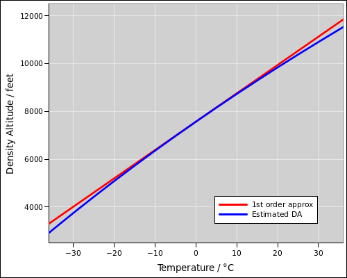
Bottom line up front: If you can measure the pressure altitude and the temperature, you can estimate the density altitude, assuming the humidity is not too high. Specifically: If the temperature is higher than standard, the density altitude is higher than the pressure altitude, by 120 feet per degree C.
It is easy to measure the local pressure altitude using an aircraft altimeter: If you set the Kollsman window to 29.92 then the dial reading is the pressure altitude. Call this hm, were the subscript “m” indicates measured.
This pressure corresponds to a particular point in the standard atmosphere. This point has a pressure Ps, density ρs, and temperature Ts, where the subscript “s” indicates standard. These values are consistent with the ideal gas law, because of how the ISA is defined.
Under standard conditions, the actual density and temperature would be ρs and Ts, but let’s consider nonstandard conditions. That is, we measure the temperature and find that it is nonstandard, i.e. different from Ts. We would like to know the density, but we don’t have a convenient way to measure that, so we estimate it based on the things we can measure. The ideal gas law constrains the possibilities:
| (27) |
The second line uses the fact that we know the actual pressure P is equal to Ps, because we just measured it. The equation tells us that when the pressure is known, a 1% increase in temperature corresponds to a 1% decrease in density.
We can plug that into equation 26, to obtain a formula for the density altitude in terms of the pressure altitude and temperature, for dry air:
| (28) |
As always, the temperatures here are absolute temperatures (kelvin, not centigrade). We can obtain a useful first-order approximation by taking the exterior derivative:
| (29) |
In words: If the temperature is higher than standard, the density altitude is higher than the pressure altitude, by 120 feet per degree C.
To use this formula, you need a measurement of the temperature, a measurement of the pressure altitude, and a chart or formula that tells you the standard temperature at that altitude.
Note this assumes dry air. If the absolute humidity is high, as it commonly is in the summer, the density altitude could be even higher than this formula suggests.
The first-order approximation in equation 29 assumes that the temperature deviation is small compared to the absolute temperature (on the order of 300 K), which it usually is. Compare the red line to the blue curve in figure 1.
Example: Suppose you are sitting on the runway at Aspen. The true altitude is 7838 feet MSL. However, due to a fluke of weather, the pressure altitude is only 7575. The standard temperature at that altitude is very close to freezing. Depending on the actual temperature, the density altitude could be quite a bit higher or lower than the pressure altitude. Note that temperatures of +30 or −30 centigrade are rare but not impossible at Aspen.
Beware: Confusing lapse-rate terminology; see remark 3.
Beware: Confusing lapse-rate terminology; see remark 3.