(If you work hard enough you can make a non-reciprocal device, such as a circulator, but it’s hard to imagine this happening by accident.)
Reciprocity applies on a frequency-by-frequency basis. In contrast, it is possible, and indeed rather common, for something to be a good antenna at one frequency and a bad antenna at another frequency. Dye molecules are a spectacular example.
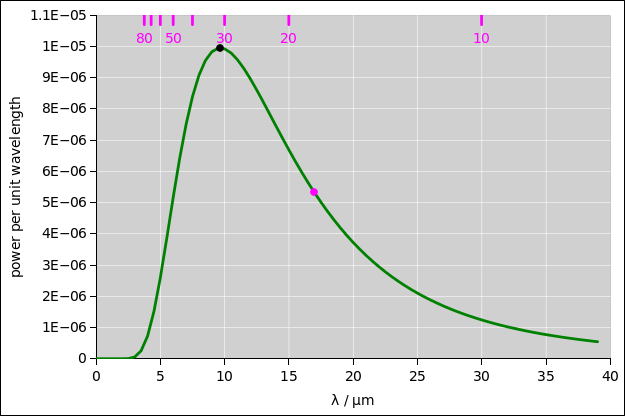
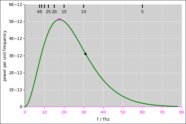
| The peak in figure 1 is at λpeak = 9.66 µm. (This is for T=300K.) | The peak in figure 2 is at fpeak = 17.6 THz. (Again for T=300K.) |
These two peak-positions represent seemingly-similar concepts (“the” peak of “the” spectrum) ... but they do not obey the formula λpeak · fpeak = c. In particular:
They’re off by almost a factor of 2. That’s because they are measuring different things. One of them is power per unit wavelength (dP/dλ) and the other is power per unit frequency (dP/df) The denominators are different, and the relationship between the denominators is nowhere near constant. You can convert from one to the other super-easily, by multiplying or dividing by a factor of dλ/df.
| The magenta tick-marks at the top of figure 1 are equally spaced in frequency units, with frequency increasing right-to-left; they correspond to the magenta tick marks on the axis at the bottom of figure 2. | The black tick-marks at the top of figure 2 are equally spaced in wavelength units, with wavelength increasing right-to-left; they correspond to the black tick marks on the axis at the bottom of figure 1. |
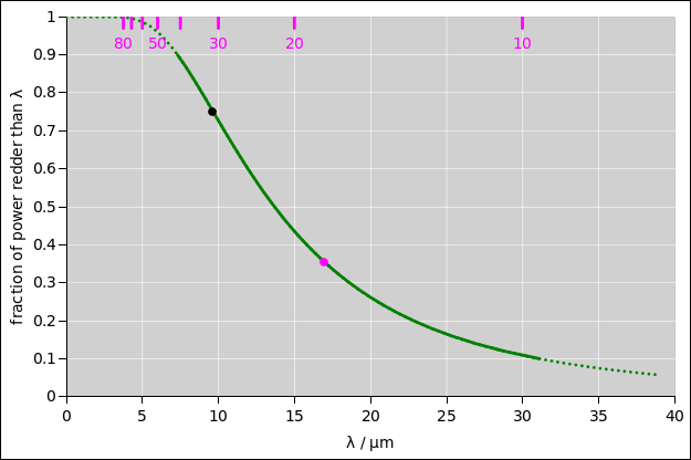
Plotting the cumulative power gives us another way to see what’s going on: Note that figure 3 uses the exact same ordinates as figure 4. We have just plotted the same ordinates against different abscissas. In particular, the height of the black dot is the same on both curves, and the height of the magenta dot is the same on both curves. We can convert one curve to the other by a simple topological distortion of the horizontal axis.
This sameness of ordinates does not persist when we differentiate to obtain figure 1 and figure 2. That’s because we are differentiating with respect to different variables!
|

| |
| Figure 3: Black Body Cumulative Power versus Wavelength | Figure 4: Black Body Cumulative Power versus Frequency | |
We can connect these figures to the previous two figures as follows:
| The black dot marks the steepest part of the curve, corresponding to the peak in figure 1. About 75% of the power is found at longer wavelengths than this (i.e. lower frequencies, i.e. colors deeper into the infrared). | The magenta dot marks the steepest part of the curve, corresponding to the peak in figure 2. About 35% of the power is found at lower frequencies than this (i.e. longer wavelengths, i.e. colors deeper into the infrared). |
The best way to quantify the breadth and lopsidedness is to look at the cumulative power.
| Figure 3 is the integral of figure 1. You can see that 80% of the power is between 7 µm and 31 µm, as indicated by the non-dotted part of the curve ... whereas 10% of the power is below this band and 10% is above. | Figure 4 is the integral of figure 2. You can see that 80% of the power is between 10 THz and 41 THz, as indicated by the non-dotted part of the curve ... whereas 10% of the power is below this band and 10% is above. |
In both cases, the width of the band is larger than the abscissa of the peak, which tells you that it is exceptionally broad. (In contrast, if the spectra were sharply peaked, these cumulative distributions would look more like step functions, less like gradual ramps. The width would be small compared to abscissa of the peak.)
The spreadsheet used to prepare these figures is in reference 1.
If something is sufficiently thin and/or dilute, you can see right through it. If you point a pyrometer at a roomful of air, it won’t measure the air; it will measure the wall or whatever it sees behind the air.
If something is sufficiently shiny, it won’t radiate appreciably. It is neither a good receiving antenna nor a good transmitting antenna. If you point a pyrometer at a shiny surface, it won’t measure the surface; it will measure whatever object it sees reflected by the surface.
It is common for an object to be shiny at one frequency, transparent at another frequency, and absorptive at another frequency.
Terminology: The term “black” usually means that the object is absorptive at all frequencies of interest. Exception: “shiny black” means you get a small amount of specular reflection when the angle of incidence equals the angle of reflection ... and absorption at other angles.
Suppose in the foreground there is a cold object that is transparent at some wavelengths and absorptive in another ... in other words, a colored filter. In the background there is a hot, glowing source. If you look through the filter toward the source, what you see is not a black-body spectrum. It is part of one spectrum plus part of another. It cannot be described by a color temperature or any other kind of temperature. This is not a thermal-equilibrium situation.
You can easily wind up with a spectrum with multiple peaks, or with notches, as in figure 5. For a much more extreme example, see reference 2, especially figure 1 therein.
Flames commonly produce spectra that are not even remotely black-body spectra. Similarly, if you see green light coming from an LED, that is not a black-body spectrum. You use it to infer the temperature of the LED. There is no such thing as a “green” color-temperature anyway.
If you point an IR thermometer at a non-thermal distribution, the results will in general be meaningless. You cannot assign a temperature to something that does not have a well-defined temperature.
In contrast, if you want to measure something small and close, you would be much better off refocusing the thing. You want the image of the detector to fall on and within the object you are measuring. To say the same thing the other way, you want the image of the object to cover the detector.
If the focusing is not perfect, and/or if the object is not a perfectly black absorber, you need to be super-careful about stray light. Control the background behind the object. Consider putting a field stop somewhere in the optical path. If the object is shiny to any appreciable degree, you basically have to enclose it completely.
| wavenumber | wavelength | |||||||
| cm−1 | µm | |||||||
| far IR | 5 | — | 500 | 2000.000 | — | 20.000 | ||
| mid IR | 500 | — | 4000 | 20.000 | — | 2.500 | ||
| near IR | 4000 | — | 14000 | 2.500 | — | 0.714 | ||
Room temperature black-body radiation is mostly in the “mid IR” band. See reference 4.

It’s hard to find plots that cover the region beyond 5 µm. As a general rule, absence of evidence is not evidence of absence, but in this case I’m pretty sure that if there were any nonzero transmission in the mid-IR they would show it on the plots.
Beware that “no transmission” does not necessarily mean black. It’s probably shiny, like a shiny black piano, and therefore not a good target for an IR thermometer. To make it really black probably requires an anti-reflection coating. Note that making a broadband AR coating is not easy.
Roughening the surface might help. Depending on details, it might result in a matte black surface. This might make it work OK as a target for an IR thermometer.
It should be easy to test all this. Measure the amount of reflection, using a nice flat piece of glass, before and after various surface treatments.