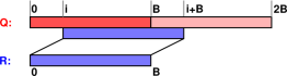
Figure 1: Lagged Dot Product
We are interested in data that comes from a photon-counting experiment. Let’s use the following notation.
| (1) |
I don’t claim that the intensity I as defined this way is always well behaved. It could look like a collection of delta functions. But this isn’t going to cause problems with what we are doing today. Everything said here in terms of I(t) could be said more precisely in terms of M(t) and ΔM, but I will also express things in the more familiar I(t) notation when possible.
The integral of the intensity is well behaved. Over any interval [t1, t2] we can write:
| (2) |
This allows us to define the average intensity. Over the interval [t1, t2] we have:
| (3) |
In the raw data as recorded in the lab, the time is quantized in bins. In any particular data set, the bin-size is constant. If/when we choose to perform coarse-graining, a grain will consist of one or more bins; we get to adjust the grain size during the analysis.
Next, we introduce the notion of zone. Each zone extends for a time T. In particular, the primary zone covers the time from 0 to T. The zone may or may not span all of the recorded data.
Let B denote the number of bins in the zone. That is:
| (4) |
The bins are discrete, and are associated with discrete times ti. In the primary zone, t0 is the starting time of the earliest bin, while tB−1 is the starting time of the latest bin. We recognize tB as the ending time of the latest bin in the primary zone, but usually we choose to identify bins by their starting time, not ending time. Of course tB is the starting time of the earliest bin in the next zone.
In symbols:
| (5) |
These quantities uphold the obvious sum rules:
| (6) |
So far we have been considering a “generic” data set M. If there are multiple data sets (for example Q and R), we need to specify which one we are talking about. We use square brackets for this (for example M[Q], M[R], J[Q], J[R], et cetera). We sometimes use subscript notation as a shorthand to refer to the binned data:
| (7) |
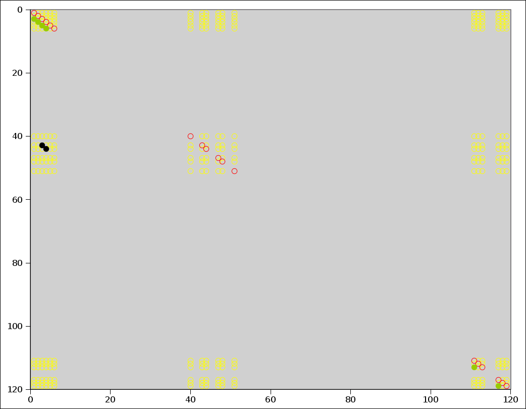
The correlation function is defined as a collection of lagged dot products. The situation is diagrammed in figure 1. The vectors Q and R are binned data, as defined by equation 7.
For a cross-correlation, the vectors Q and R are different, whereas for an autocorrelation, R is a copy of the primary zone of Q.
From now on we will need to be careful about boundary conditions.
| (8) |
The raw correlation function (RCF) as computed by the low-level software is
| (9) |
Our understanding of the physics leads us to expect Qk to be statistically independent of Qk−i for moderately large i (and for all k). We need to be careful how we use this fact, because independent (in the sense of statistics) is not the same thing as uncorrelated (in the sense of autocorrelation function), for reasons we are about to discuss.
Because of the possibility of statistical independence, we are motivated to consider the fluctuations δJ relative to the average ⟨J⟩. Therefore we define:
| (10) |
where ⟨Q⟩ was defined in equation 5 and we are using the shorthand introduced in equation 7. This δQ obeys the obvious sum rule
| (11) |
Plugging this into equation 9 we get
| (12) |
For periodic boundary conditions, the two cross terms (the two middle terms in equation 12) are strictly zero, and the last term reduces to
| (13) |
In the wings, where we expect things to be statistically independent, it is “conventional wisdom” to assume that the first term in equation 12 is well approximated by zero. For reasons that will become clear in a moment, we call this the ftK approximation (“flatter than Kansas”). It is, alas, not always a satisfactory approximation.
The ftK approximation – i.e. ignoring first term in equation 13 – would be provably OK if there were no correlations anywhere, but given that we do have correlations when the lag is small, this term cannot be neglected, even in the wings. A pair of numerical scenarios should suffice to prove this point:
In the first scenario, we have data that is as smooth as it could possibly be, without even any Poisson noise, just uniformly distributed. In particular, suppose we have B=10 bins with one photon per bin. That implies ⟨Q⟩=1 and δQi is identically zero. The autocorrelation is equal to 10 for all i, and the value in the wings is equal to B⟨Q⟩=1 as given by the last term in equation 13 as expected.
The second scenario is the same as the first, except that on top of the uniform background, there is an additional bunch of 10 photons in one of the bins. It doesn’t matter which bin; let’s say bin #7 just to be definite. The average is now ⟨Q⟩=2 and δQi=−1 in the wings, i.e. everywhere except for zero lag. The autocorrelation function is equal to 130 at zero lag, and equal to 30 everywhere else, which is distinctly different from the value (40) lamely suggested by the last line of equation 13.
If we boldly make the ftK approximation anyway, it explains the following so-called conventional wisdom: Suppose you are using boundary conditions and you want to construct a cooked correlation function (CCF) where the wings are invariant with respect to changes in bin-size. Then you should divide the RCF by T2/B [ftK only]. Similarly, if you want the CCF to be normalized so that it goes to 1 in the wings, you should divide the RCF by ⟨I⟩2T2/B [ftK only].
Here is an easy way to understand, qualitatively, the normalization that is “conventionally” applied to the RCF. The essential physics is independent of bin size. The bin size is introduced artificially by the processing algorithm, and we want to normalize things so that the bin size drops out. The physics is well represented by I(t) and M(t) which are independent of bin size, in contrast to Ji which is not independent of bin size. Alas the low-level software operates on the Ji values. A factor on the order of T2/B is needed to make the results independent of bin size.
In any case, keep in mind that this “conventional” factor of T2/B is not entirely satisfactory. The alleged result fails miserably for dark boundary conditions, and is dubious at best for periodic boundary conditions. In this-or-that experimental situation the discrepancy might be below the noise, but then again it might not. A more detailed analysis is required. Section 2 takes a few further steps down this road.
In this section, we try to understand what’s going on with the normalization of the wings of the correlation function, with particular attention to dark normalization. I don’t entirely understand how to quantify this. In particular, intuition and a conceptual physical argument suggest that the data in the wings should be – in some sense – statistically independent, but I am not yet sure how to quantify this in terms of correlation functions. So for now the next step is to tee up the problem in reasonably clear terms so it can be discussed.
We can do this with the help of figure 2.
We are (for the moment) using dark boundary conditions. Therefore the correlation function value CF(i) is a sum over B−i cells. We call i the lag, since CF(i) is a lagged dot product.
In the figure, the red hits are on the diagonal. They contribute to the zero spike, i.e. the value of the correlation function at zero lag. There are 18 such hits, so that CF0 = 18. The green hits are two units below the diagonal, so they are associated with a lag of 2. There are six of them, so CF2 = 6. The black hits are 40 units below the diagonal, and there are 2 of them, so CF40 = 2.
In the entire XY space shown in the figure, there are N2 hits spread over B2 cells. If we temporarily assume the hits are approximately evenly distributed over the cells, then CFi is approximately (B−i)N2/B2 = (1−i/B)N2/B. If we are not too far from the diagonal this can be further approximated as simply N2/B.
There will be statistical uncertainty in the correlation function values, just due to the luck of the draw as to where the hits fall in the XY space. The absolute uncertainty in CFi will be at least √CFi which corresponds to a relative uncertainty of 1/√CFi.
At the level of dimensional analysis, it makes a certain amount of sense to normalize the correlation function values by dividing by N2(B−i)/B2 or (1−i/B)N2/B. This makes more sense than not normalizing at all. In addition to the normalized value, we must also keep around the un-normalized value, because we need it for calculating the statistical uncertainty.
This choice of normalization does not mean that the tail of the correlation function will converge to 1. Here’s why: We know the hits are not evenly distributed over the XY square depicted in figure 2. There is a heavy concentration near the diagonal. Therefore the off-diagonal regions will be depleted relative to the globally-average value.
In more detail: Suppose there are N total photons grouped into C clumps, where each clump has a width of roughly w in the time direction. There are roughly N/C photons per clump. In figure 2 there will be C clumps near the diagonal, with N2/C2 hits per clump, for a total of N2/C hits near the diagonal, i.e. where the lag i is less than w. That means there are N2(1−1/C) hits in the (B−w)2 cells not near the diagonal, for an average of N2(1−1/C)/(B−w)2 hits per cell. So the expected value of CFi is:
| ⟨ CFi ⟩ = N2(1−1/C)(B−i)/(B−w)2 (14) |
In the common case where B is huge, we can neglect w, so this reduces to N2(1−1/C)(1−i/B)(1/B).
You might think that we could also neglect the (1−i/B) factor, but if you run out the baseline (as you should) and use a large bin size (as you should), the relative uncertainty in the correlation function values gets very small, and a correction of the order of i/B is large compared to the uncertainty, even if it is still smallish in absolute terms. This is called the “short sum” correction, since it has to do with the fact that the number of terms in the sum that defines the correlation function decreases as i increases. You can make it go away entirely by imposing periodic boundary conditions.
So we expect the tail of the normalized correlation function to converge to something slightly less than 1. As the total time of the recording increases, the number of clumps increases, and 1−1/C converges to 1 from below.
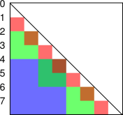
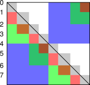
Accounting for short sums can be slightly tricky if you coarse-graining the data, and the grain-size is changing as you go along. The situation is shown in figure 3. We start with a histogram containing 8 bins and calculate the correlation. The red squares all have a grain-size of 1 and a lag of 1. The sum over these red squares is CF(1). Note that the first red square is centered at 1.5, but that represents a lag of 1.0, not 1.5, since it is exactly 1.0 below the diagonal. Meanwhile, the green squares all have a grain-size of 2 and a lag of of 2. The sum over these green squares is approximately CF(2). Specifically, it is a coarse-grained version of CF(2). All the blue squares have a grain-size of 4 and a lag of 4. The sum over all these blue squares is a coarse-grained version of CF(4).
The idea of using a grain-size that changes from time to time within the zone is called a multi-tau analysis. Reference 1 is an early example of this. Schemes where the grain size grows more-or-less exponentially are called pseudo-geometric series.
It is amusing that the grains do not overlap long the X-axis and do not overlap along the Y-axis, but they do overlap in XY space. This overlap would never have occurred if all grains had been the same size.
A variation on this is shown in figure 4. In this case we take two steps of a given size before switching to a new size. The concise way of expressing the rule is to say we have two steps per octave. Don’t worry about the gray grains; they don’t fit the pattern, but that’s OK. They are part of a startup transient, needed to start the ball rolling. This is related to the fact that we cannot extend the logarithmic pattern all the way to t=0. The logarithm of zero is not very nice. The red and green squares have a grain size of 1. The red squares have a lag of 2 and the green squares have a lag of 3. The sum of all the green squares is CF(3). Next, Next we have the blue and yellow squares, which have a grain size of 2 and lags of 4 and 6 respectively. The sum of all the yellow squares is a coarse-grained approximation to CF(6).
Again we see that the grains do not overlap in X or Y, but do overlap in XY.
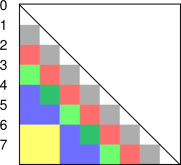
Continuing farther down this road, we come to figure 5. First we have a startup transient with grain size 1 (white,gray,green,gray). Next comes a group of four that follows the pattern; the rule in this case is 4 steps per octave, which has twofold finer resolution than the rule used in the previous example. The squares in this octave (green,red,green,red) have a grain size of 1 and a lags of 4, 5, 6, and 7 respectively. The next octave also has four points per octave. (blue,yellow,blue,yellow). They have a grain size of 2 and lags of 8, 10, 12, and 14 respectively.
All this reminds of the maxim that the normalization issue and the sum-rule issue are different. The concepts overlap, but neither is a subset of the other. In this case, normalization of the grains is relatively easy, since we know the area of each grain. On the other hand, applying the sum rule is tricky because some photons are being used twice (unless we take steps to subtract off the overlap regions).
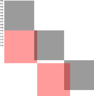
Things get ugly when the grain sizes are not commensurate. In figure 6 the gray grains are of size 10, while the red grains are of size 11. That is, the red step is 10% bigger than the gray step.
If things are evenly spaced along X and Y, they are a mess in XY space, with some photons double-counted and some not counted at all.
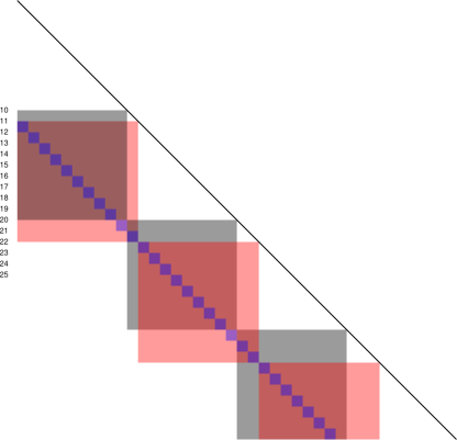
Note that the squares in figure 6 do not come anywhere near the diagonal. The first gray square starts at X=100 and ends at X=110. Contrast this with the squares in figure 7, all of which lie on the subdiagonal, such that each of them has a corner that touches the diagonal. The gray squares have a grain size of 10 and a lag of 10, while the red squares have a grain size of 11 and a lag of 11. The sum of the gray squares is a very coarse approximation to CF(10), while the sum of the red squares is a very coarse approximation of CF(11).
You can see that a large proportion of the hits are shared between the estimates of CF(10) and CF(11). The estimates will be highly correlated.
Also, because of the large grain size, the estimate of CF(11) will be heavily biased relative to the actual CF(11) as shown by the blue squares. The bias will not average out, because the density of hits in near the diagonal is much higher than the density of hits farther from the diagonal.
The previous section considered what happens if the grains at any particular lag are all the same size, but this size is not commensurate with the grain-size for some other lag.
Now we turn to a different issue. We consider the case where at a given lag, the grains are slightly uneven, i.e. not all the same size. We shall see that this does not prevent us from making the grains at this lag commensurate with the grains at other lags.
Uneven grains have been considered before, e.g. in reference 2.
Uneven grains can arise from the following situation: Suppose you want to divide 100 events into 8 grains. This can be done using slightly uneven grains (12,13,12,13,12,13,12,13). One alternative would be to use 8 grains of 12, which would require discarding the half grain that is left over at the end. A slightly-better alternative would be to spread out the discards more evenly, e.g. (12,12,x,12,12,x,12,12,x,12,12,x) where “x” represents a discarded event. Both alternatives are distasteful, because I generally don’t like discarding data if there is a viable alternative.
An example of uneven grains is shown in figure 8. The cells on the diagonal are square. Many of the off-diagonal cells are rectangular.
The interesting thing is the rule for combining things when we go from one resolution to the next. The width of each green cell is the sum of the widths of the two red boxes that occupy the same X-coordinates Similarly, the height of the green box is the sum of the heights of the two red boxes that occupy the same Y-coordinates. This is a generalization of the rule that produced figures such as figure 3.
As before, there is some slight double-counting of events, but this is no worse than what we saw previously, e.g. figure 3.
Using uneven grains requires redoing the theory that led to equation 14, since B is no longer a constant, but this should be easy to do.
In figure 8, unlike previous figures, I snuck in some additional cells that represent periodic boundary conditions (if we choose to include them in the sum). These are the cells above the diagonal.
Periodic boundary conditions do not solve all the world’s problems.
In particular, some events are left uncounted, as you can see from the white areas in the figure. Alas these uncounted events do not correspond to or compensate for the doubly-counted events. So we have a bit of a mess. I haven’t figured out how to understand this.
The main appeal of periodic boundary conditions is that it makes the short-sum problem go away. That doesn’t seem like a big-enough advantage. Right now, unless somebody has a better idea, I’m leaning toward using non-periodic boundary conditions, and factoring in the short-sum correction, which is easy to do.
It is also not entirely obvious how to determine "the" period, due to limitations of the raw data format we are using. The data was sampled over some time-span. We know that the span begins at t=0, but we don’t know when it ends. All we know is the time of the last event. We don’t know how much "dark lead-out" time there was following the last event.
// Suppose we have a conceptual vector with
// 9 bins labeled 0 through 8 inclusive
//   +----+----+----+----+----+----+----+----+----+
//   |0   |1   |2   |3 * |4   |5 * |6   |7   |8   |9
//   +----+----+----+----+----+----+----+----+----+
//   [-- lead_in  --]              [-- lead_out --]
//
//  record_first   = 0
//  record_last    = 8 = (N-1) = not very interesting
//  N == span_bins = 9 = 1 + last_event + lead_out
//  span_time      = N*dt
//  first_event    = 3
//  last_event     = 5
//  lead_in        = 3
//  lead_out       = 3 by heuristic construction;  not recorded by instrument
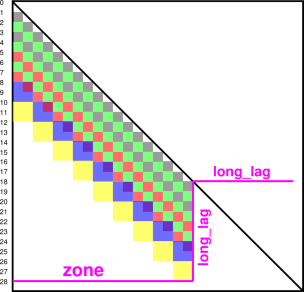
Consider the situation shown in figure 9.
For extended boundary conditions, the zone size must satisfy three conditions:
Each of these three points can be seen in the figure, if you look closely enough. There are 29 data points total, for both X and Y, numbered 0 through 28 inclusive. The last data point never gets used at all, because it is a remainder when we quantize things to a multiple of the largest grain.
Note that in this figure, X runs vertically and Y runs horizontally. Sorry.
The longest lag in this example is 10 units. We use 28 of the X data points, but only 18 of the Y data points. We must sacrifice the rest of the Y data points in order to implement extended boundary conditions. The zone size is 18.
Actually, given a X-span of 29 and a long_lag of 10, any Y-span from 18 to infinity inclusive would produce the same result.
Note that we do not have a full octave’s worth of the largest grains. There are only two grains in this octave, whereas a full octave would have four. This is based on an arbitrary decision about how long we want the longest lag to be, i.e. how wide is the “band width” of the band of cells near the diagonal. This has got nothing to do with the span of the data; the data span could be 29 or it could be 1,000,029 and the band width and grain sizes would be the same.
For any given run of the correlator, the X and Y data are not treated symmetrically, because only the X data gets lagged. On the other hand, when doing cross correlations, it is advisable to exchange the roles of X and Y and re-run the correlator. For an auto correlation, this would be a waste of time, because the second-run output would be identical to the first-run output. However, for a cross correlation provides new information.
The following two figures are derived from the 04102010_Alexa013.pt2 dataset. They are the same except for the fineness and the sign of the lag, which varies as specified in the captions.
It is interesting to compare this with the auto correlation data for the same dataset, shown at the beginning of section 7.
In all cases, the abscissa is the common log of the lag, where the lag is measured in seconds. The ordinate is the correlation function, normalized so that it goes to 1 in the wings.
04102010_Alexa013f4xy.pt2, 4 Points Per Octave
04102010_Alexa013f8xy.pt2, 8 Points Per Octave
04102010_Alexa013f8yx.pt2, 8 Points Per Octave,
Negative Lags
The following figure is derived from the 04102010_Alexa013.pt2 dataset. You can compare it to the cross correlation results in section 6.
The following three figures are derived from the data007.dat dataset, for which only auto correlation is possible. They are all the same except for the fineness, which varies as specified in the captions.
data007.dat, 4 Points Per Octave
data007.dat, 8 Points Per Octave
data007.dat, 16 Points Per Octave