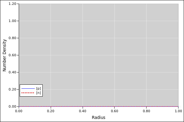
Figure 1: Number Density versus Radius, Rough Starting Point
Imagine a spherical droplet containing some electrolyte. That means there are some dissolved ions. For the moment, for simplicity, we assume only two species of ions, perhaps Na+ and Cl−.
We assume radial symmetry. We work in spherical polar coordinates. We use the following variables:
| (1) |
Then the relevant equations include, for each species:
| (2) |
| (3) |
We can eliminate the diffusion constant in favor of the mobility (or vice versa) using the Einstein-Smoluchowski relation:
| (4) |
We will also need Gauss’s electrostatic law:
| (5) |
We solve the equations by finite element modeling. We divide the droplet into N concentric shells, labeled 1 through N inclusive. There will be N+1 boundaries, labeled 0 through N inclusive. Of these, N−1 will be “ordinary” boundaries between adjacent shells. Boundary #0 is the degenerate zero-sized “boundary” at r=0. Boundary #N coincides with the edge of the droplet. It is exceptional, because it is where we impose the boundary conditions. Among other conditions, we assume no current can flow through this boundary.
For each and every ordinary boundary, we calculate the current across the boundary. We then time-step the equation.
We choose units of length such that the droplet has unit radius.
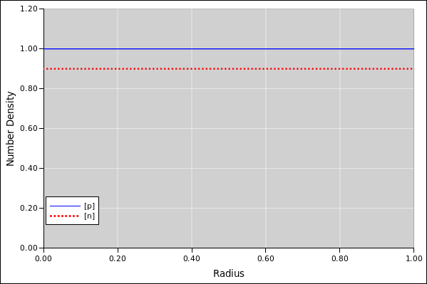
As a first example, suppose the droplet contains 4π/3 units of the positive species, so the average density is unity. The droplet also contains the same amount of the negative species. However, 10% of the negative species is stuck to the outer boundary, so only 0.9 units is floating around in the bulk.
The results of the simulation are shown in the following figures. We can initialize the iterative calculation by setting the number-density of each species to be uniform in space. This is not the equilibrium distribution; it is just a rough starting point.
In accordance with equation 4, setting the diffusion constant to zero is equivalent to setting the temperature to zero. Let’s take a look at that.
In figure 2 we see that some of the positive charges move to the outside of the droplet and establish a dipole layer. This is unsurprising, since they are repelled by each other, and attracted to the negative charge at the boundary. Similarly some of the negative charges are repelled from the boundary. In the bulk, there is zero net charge density; the bulk distribution is compensated, i.e. it has equal amounts of positive and negative charge. There is no electric field in the bulk. The charge trapped at the boundary is fully screened.
We now switch to finite temperature. We choose a diffusion constant that is one tenth of the mobility, in units where kT=1.
In this case, as you can see in figure 4, there is nothing we would recognize as a dipole layer. Due to diffusion – or, equivalently, due to thermal agitation – the charges spend essentially all of there time somewhere in the interior. The positive charges exhibit only a modest tendency to concentrate near the outside. The free negative charges are only moderately depleted near the outside.
There is a substantial electric field extending into the interior. The field is not well screened, even with this rather modest amount of diffusion.
Indeed, in figure 6 you can see that most of the volume sees most of the electric field.
The spreadsheet used to product these figures is in reference 1.
Brute-force time-stepping is remarkably ill-behaved, unless the time-step is rather small. On the other hand, since we are doing a one-dimensional simulation with a small number of shells, we can afford a tiny time-step.
To use the spreadsheet, start by setting and then unsetting the reset button. Click to set, then click to unset. The spreadsheet will do one iteration of the calculation. Hit F9 to cause more iterations. Hit F9 as many times as you like. Eventually the calculation should converge. Watch the graphs to see the equilibrium distribution emerge. If the calculation diverges, reduce the timestep, hit reset, and start over.
Suppose we model the equilibrium charge distribution as follows: We divde the droplet into a crust of zero thickness, surrounding a mantle of thickness 2λ, surrounding an inner core. The rationale for that factor of 2 will become apparent soon. The goal of this section is to determine a value for λ. Hint: Subject to a few mild assumptions, it will turn out to be the Debye screening length.
We imagine that in the mantle, the charge density starts at some maximum value ρ* at the outer edge and goes linearly to zero, reaching zero at the mantle/core boundary. We know it is actually more like an exponential, but we approximate it by a straight line.
There is some charge −Qt trapped in the crust. This is a surface-charge density. This charge is screened by an excess of positive species and a deficit of negative species in bulk within the mantle. The total charge in the mantle is +Qt.
By the time we get to the core, everything has been fully screened. In the core, there is no electric field. The positive species are compensated by the negative species.
Consider the situation at mid-mantle, i.e. at a point where r = R − λ. Approximately half of the bulk charge is inside this point, and half outside. Therefore by Gauss’s electrostatic law,
| (6) |
The dielectric constant does not appear in this expression. It depends only on the continuity of flux lines, which is not affected by a dielectric.
We can integrate the field to find the voltage.
| (7) |
Hence the effective capacitance is
| (8) |
Here’s another way to think about this capacitor. Imagine the inner plate is at the mid-mantle point. The effective area is 4π(R − λ)2. There is capacitor gap of λ between mid-mantle and crust. The idea here is that an electric field line originates on a positive charge somewhere in the mantle and terminates on a negative charge trapped in the crust.
Assuming R ≫ 2λ, the capacitance of this pecular capacitor is:
| (9) |
in agreement with equation 8.
We assume the voltage V on this capacitor is some more-or-less known constant, representing the chemistry of whatever is trapping charge in the crust. We express the charge as Qt = CV, so that is known as a function of λ. At this point we still have only one unknown, namely λ.
The number of field lines that originate in the mantle is just Qt/e. Equivalently, this is the number of uncompensated ions in the mantle. The average number density is
| (10) |
and the peak number density is twice that. The concentration gradient and diffusion current are:
| (11) |
Meanwhile, the electrical drift current is
| (12) |
where this ρ is the nominal concentration of sodium chloride, and 2ρ is the the total number of ions, not just uncompensated ions. The electric field drives all of the positive ions one way, and all of the negative ions the other way. This depends on the total concentration, in contrast to diffusion, which depends only on the concentration gradient. If you overlook this point, you will get the wrong answer, wrong by a factor of δρ over ρ.
To say the same thing another way, drift depends on [p + n], which you could get by adding the blue and red curves in figure 4, so it is roughly twice the height of either curve ... whereas diffusion depends on the splitting between the blue and red curves, which in some cases of interest is considerably smaller.
We need the factor of the dielectric constant єr in equation 12, because we care about the energy required to move an ion from capacitor plate to the other, and this is reduced by a factor of єr.
In equilibrium, the two currents are equal, so
| (13) |
We identify λ as the Debye screening length.
Under the action of mobility alone (aka electrostatic forces), λ would shrink to zero, resulting in a super-thin dipole layer. Under the action of diffusion alone (aka thermal agitation), λ would grow large, resulting in a uniform charge density.
The Bjerrum length scales inversely with kT, and depends not at all on concentration. This stands in contrast to the Debye length, which increases with increasing kT, and decreases with increasing concentration.
You can construct the Debye length in terms of the Bjerrum length and the molar volume, but in the present situation, as far as I can see, that’s just numerology, not physics.
The mobility for other species can be inferred from the relative mobilities in reference 5. A few of the required multiplications are carried out on one of the tabs in reference 1.
At low concentrations (low compared to normal saline) all sorts of peculiar things happen.
For pure unbuffered water, if you think there is a a definite number of OH− ions, a huge fraction of the OH− will wind up trapped in the crust. So, in the bulk one might imagine very little OH− and a huge concentration of H+ ... but this cannot possibly be what happens. It would violate conservation of charge.
I need to think about it some more, but I assume what happens is that water dissociates to make more OH− ions, partially replacing the ones that got trapped in the crust.
Imagine that there is a N-to-1 ratio of OH− in the crust relative to in the bulk. Then in the bulk [OH−][H+] = constant, and [H+] is larger than its pure-water value by a factor of √(N+1), while [OH−] is less than its pure-water value by the same factor. If this analysis is correct, it means the pH in the bulk goes down, but maybe not as much as one might have guessed. For n=10000, the pH goes down by 2 units, i.e. log10(√10001).
The increased concentration of H+ would make λ smaller than it might have been, except that λ is stuck at R in this regime.