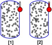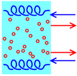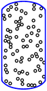
Figure 1: Tank of Gas
In order to get some appreciation for the basic gas laws, let’s start by considering some simple experimental scenarios. We will measure the pressure, volume, temperature, etc. of gases in various situations. Different scenarios involve different choices of experimental conditions.
We start with a big tank, as shown in blue in figure 1. Within the tank are a number of gas particles (shown in black). In all scenarios considered here, we assume the gas can be satisfactorily approximated as an ideal gas. This is a reasonable approximation for gases such as air under everyday conditions.
Also, we choose to hold constant the number of gas particles (N). In most scenarios, we need not make any assumptions as to whether the particles are molecules and/or individual atoms.
We adopt the usual notation:
| P | ≡ | pressure |
| V | ≡ | volume |
| T | ≡ | temperature |
| S | ≡ | entropy |
| N | ≡ | number of particles |
| k | ≡ | Boltzmann’s constant |
| N′ | ≡ | number of moles of particles |
| R | ≡ | universal gas constant |
Boltzmann’s constant (k) is a universal constant that defines what we mean by one “degree” of temperature. It is the conversion factor that converts from degrees to conventional units of energy per particle. It is intimately related to the universal gas constant (R) which converts from degrees to conventional units of energy per mole.
| k | = | energy per particle |
| R | = | energy per mole |
That means we can write the ideal gas law in two ways:
| (1) |
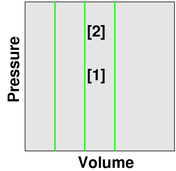
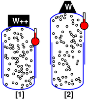
In our first scenario, as indicated in figure 2, we choose to make the tank sturdy and leak-proof. That means the number of particles does not change, and the volume does not change.
We investigate the effect of temperature. We observe that as the temperature goes up (as indicated by the little thermometer icons), the pressure goes up. In figure 3, the point describing the system moves from point [1] to point [2] along a contour of constant volume. (This is also a contour of constant number of gas molecules, N, but the N variable is not shown in the graphs.)
This scenario can be described mathematically as follows:
| (2) | ||||||||||||||||||||||||||||||||||
Equation 2 is to be interpreted as follows: The ideal gas law (P V = N kT) is common to all ideal-gas scenarios. The other equations are much less general, and are valid only within this scenario.
The first line of equation 2 is a system of three equations that suffice to describe this scenario. The second line is a corollary of the first, and also suffices to describe this scenario. The first line has one general equation and two scenario-specific equations, while on the second line all three equations are scenario-specific.
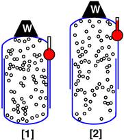
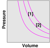
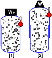
For our next scenario, we choose a modified container, designed to keep the gas at constant pressure rather than constant volume. One part of the container is free to slide relative to the other part. There is a weight W on the top part, to supply the desired amount of pressure.
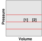
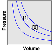
We observe that as the temperature increases, the volume increases. The point describing the system moves from point [1] to point [2] along a contour of constant pressure, as shown in figure 5.
This scenario can be described mathematically as follows:
| (3) | ||||||||||||||||||||||||||||||||||
Equation 3 is to be interpreted as follows: The ideal gas law (P V = N kT) is common to all ideal-gas scenarios. The other equations are much less general, and are valid only within this scenario.
The first line of equation 3 is a system of three equations that suffice to describe this scenario. The second line is a corollary of the first, and also suffices to describe this scenario.
For our next scenario, we arrange to have “no friction” (or very little), and “no heat leaks” (or very little).
To say the same thing more formally, we want to keep the entropy constant. If you don’t know what entropy is, don’t worry about it too much right now, and follow the scenario as described in the previous paragraph.
If the tank is large, this is relatively easy to arrange; we just need to make sure the experiment is done neither too quickly nor too slowly.
If the tank is not large and not thermally insulated, the window between “too quickly” and “too slowly” may be inconveniently small (or perhaps nonexistent). Conversely, if we make the tank large enough and provide reasonable thermal insulation, there will be plenty of time to change the volume with minimal dissipation, and plenty of time to make the desired measurements.
In this scenario, we observe that smaller volume is associated with higher pressure (and vice versa). Also, the gas cools as it expands (and heats up as it is compressed). The point describing the system moves from point [1] to point [2] along a contour of constant entropy, as shown in figure 9.
This scenario can be described mathematically as follows:
| (4) | ||||||||||||||||||||||||||||
where γ (the Greek letter gamma) is the so-called adiabatic exponent. It is also called the ratio of specific heats, for reasons that need not concern us at the moment. The value of γ is 5/3 for a perfect monatomic gas, and 7/5 for diatomic rigid rotors. At ordinary temperatures, the observed value for air is very close to 1.4, as expected.
Many gases can be described by saying P V(γ) is some function of the entropy. This is usually a good approximation, provided the temperature doesn’t get too high or too low.
The first line of equation 4 is a system of four equations that suffice to describe this scenario. Actually we only need three of them; the ideal gas law remains valid but is not needed for present purposes. The second line is a corollary of the first, and also suffices to describe this scenario.
The equations grouped on the right side of equation 4 are much less general, and are valid only within this scenario.
For our next scenario, we arrange to keep the temperature constant. If the tank is large, this may require waiting a very long time for the temperatures to equilibrate. If you get tired of waiting, you can speed things up by pumping the gas through a heat exchanger, or otherwise engineering faster heat transfer.
In this isothermal scenario, we observe that smaller volume is associated with higher pressure and vice versa. The point describing the system moves from point [1] to point [1] along a contour of constant temperature, as shown in figure 9.
This scenario can be described mathematically as follows:
| (5) | |||||||||||||||||||||||||
Once again, the ideal gas law (P V = N kT) is common to all ideal-gas scenarios. The other equations are much less general, and are valid only within this scenario.
The first line of equation 5 is a system of three equations that suffice to describe this scenario. The second line is a corollary of the first, and also suffices to describe this scenario.
The term osmosis covers both osmotic pressure (section 2.1 and section 2.4) and osmotic flow (section 2.3). We start by considering osmotic pressure, since it is simpler, and since it is what we observe under equilibrium conditions.
Executive summary: The solute behaves as a gas. It pressurizes the solvent from within. This solute-as-gas model is simple, explanatory, and predictive.
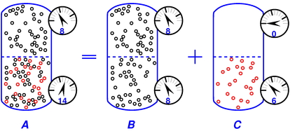
The easiest way to explain osmotic pressure is to connect it to Dalton’s law of partial pressures, as shown in figure 10.
For simplicity, we start by considering gas-in-gas osmosis. (The case of solute-in-solvent is essentially the same anyway, as discussed in section 2.4.)
The figure shows the equilibrium situation and explains it in terms of A = B + C. The rule is:
| total pressure = solvent pressure + solute pressure (6) |
Limitations: Part A of the diagram represents a measurement we can easily conduct in the lab, while the decomposition into B+C may be only a Gedankenexperiment. See section 2.7 for additional limitations on this equation.
The black particles (in both parts of the tank) have a pressure of 8 units, while the red particles (in the bottom half of the tank) have a pressure of 6 units, as shown by the pressure gauges attached to the side of the tank. Applying equation 6 to this example, we have:
| (7) |
The membrane in the middle of the vessel is permeable to the black particles but impermeable to the red particles.
We assume both the black gas and the red gas are ideal gases. That means (among other things) that the particles are very small compared to the mean free path. The figure exaggerates the size of the particles, so you will have to use your mind’s eye to imagine that the particles are very much smaller than shown.
The osmotic pressure (i.e. the differential pressure across the membrane) is simply equal to the partial pressure of the red particles, i.e. 6 units in this example.
In contrast, the partial pressure of the black particles exerts no net force on the membrane, because this pressure, whatever its value, has the same value on both sides, whenever the system is in equilibrium, as in figure 10. (You can consider this an application of Pascal’s principle if you wish.) The pressure of the black particles could be 8 units or 800 units or whatever, and it would not affect the osmotic pressure.
In part B of the figure, the semipermeable membrane can be removed entirely, leaving a wide-open connection.
In part C of the figure, the semipermeable membrane can be replaced by a solid barrier.
If you consider a particle in interior of the top compartment, there is no net force on any of the black particles. There is pressure, but at equilibrium there is no pressure gradient, and therefore no net force.
The same applies to a particle anywhere in the interior of the bottom compartment. There is red partial pressure and black partial pressure, but at equilibrium, there is no pressure gradient, and therefore no net force anywhere in the interior.
The only place in the whole system where there is any pressure gradient is right at the membrane. You can see this gradient at a glance in figure 10, especially part C of the figure, because the gradient in the pressure is associated with a big gradient in the density of the red particles.
Now the key point is that this pressure gradient is 100% "used up" in exerting a force on the membrane. There is nothing "left over" to exert a force on the black gas particles.
To make the same point the other way around, whenever an upward-moving red particle hits the membrane, it gets turned around and sent back downward (otherwise the membrane would leak, and we can’t tolerate that). Therefore at every location where a black particle might be hit by a red particle, it is equally likely to be hit by an upward- or downward-moving red particle.
In contrast, if you look at other systems you can sometimes find situations where one gas exerts an unbalanced force on another gas, such as in a diffusion pump, where you use oil vapor to exert a force on the gas you’re trying to pump. However, this is necessarily associated with flow of the oil vapor, and is therefore dissimilar to figure 10, where the red gas is not flowing.
The key idea is just a simple force-balance argument. In part B of the figure, the forces are in balance, with no force on the membrane, because the black gas moves freely through the membrane. In part C the forces are in balance, with a force on the membrane, because the red gas pushes on the membrane (and the membrane pushes on the red gas). Putting those two parts together, we conclude that there must be a force on the membrane in part A. Otherwise the forces would not be in balance.
As long as the membrane exerts a force on the red gas and not on the black gas, there will be osmotic pressure.
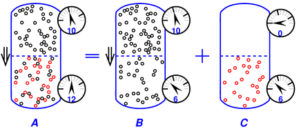
Figure 11 shows what happens in a situation far from equilibrium.
We have an imbalance (between top and bottom) of the partial pressure of the black phase. This is particularly easy to see in part B of the diagram. Since the black phase is free to flow through the membrane, it will do so, under the influence of this imbalance in partial pressure. Flow is indicated by the ⇓ arrow.
If you think about it the wrong way, this flow seems paradoxical. If you focus on the total pressure, as in part A of the figure, the black particles are flowing the “wrong” way, from lower pressure to higher pressure. The smart way to think about it is to focus on the partial pressure of the black particles by themselves, as in part B of the figure. Then you can see that the flow goes the right way, from higher partial pressure to lower partial pressure.
Let’s switch from talking about flow to talking about pressure for a moment. The pressure difference across the membrane in part B of the diagram is not due to osmotic pressure; instead it is associated with the viscous pressure drop as the fluid flows through the membrane. The pressure across the membrane in part C of the diagram is what we properly associate with osmotic pressure. The observed total pressure across the membrane – as shown in part A of the diagram – is the sum of these two contributions A=B+C (with due regard for signs).
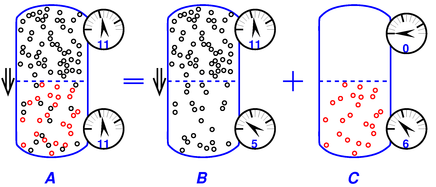
Figure 12 is similar to figure 11, but shows the special case where the non-osmotic contributions to the pressure drop are equal and opposite to the osmotic pressure, resulting in zero overall pressure differential across the membrane. This is an important special case, because it frequently arises in practice. In this case we cannot easily observe the osmotic pressure, but we do observe osmotic flow.
If you start with figure 12, it will spontaneously evolve to figure 11 and then asymptotically to figure 10.
You can see that osmotic flow is more complicated than osmotic pressure. The equilibrium situation has osmotic pressure, with no flow.
In figure 10 we can call the red particles the solute, and call the black particles the solvent. In section 2.1 we imagined that the solvent was a gas, i.e. we had one gas dissolved in another, but in this section we imagine that the solvent is a liquid. It turns out that it really doesn’t matter whether the solvent is a liquid or a gas, assuming we are dealing with an ideal solution. (In general, an ideal solute is profoundly analogous to an ideal gas.)
As before, the membrane is permeable to the solvent, so the solvent exerts zero differential pressure on the membrane.
As before, the osmotic pressure is simply equal to the partial pressure of the red particles.
There is a well-known formula for the osmotic pressure, namely
| Π = i M R T (for an ideal solution) (8) |
where Π is the osmotic pressure, M is the molarity of the solute, T is the absolute temperature, and R is the universal gas constant (i.e. Boltzmann’s constant in the appropriate units). We shall discuss the factor of i in a moment.
Equation 8 is often called the van ’t Hoff equation in honor of Jacobus H. van ’t Hoff. (Beware that there is another equation that is also called the van ’t Hoff equation.) The same equation is also called the Morse equation, in honor of Harmon Northrop Morse ... even though it was first derived by van ’t Hoff.
The astute reader will have noticed the correspondence between the ideal gas law (equation 1) and the osmotic pressure law (equation 8), provided we interpret iM as corresponding to N/V, the number of particles per unit volume in the solution. Of course this correspondence is not a mere coincidence; the osmotic pressure must be equal to the partial pressure of the solute, for good fundamental reasons.
The factor of i is necessary because of the conventional definition of the molarity M, which has to do with the number of formula units in solution, whereas the pressure depends on the number of particles.
Note that the idea behind this factor of i applies to gases as well as solutions. That is, the N that appears in the ideal gas law is the number of particles, not the number of formula-units in the gas. As a specific example, under some conditions we can have a gas of acetic acid monomers, CH3COOH, whereas under slightly different conditions we can have a gas of dimers, (CH3COOH)2. If the number of moles of acetic acid formula units is the same in both cases, the N that appears in the ideal gas law – i.e. the number of particles – will be half as great for dimers. That is, we can write N/V=iM, where i=½ for dimers.
Also note that the size of the particle is not relevant to the pressure. A large sugar molecule has the same effect as a tiny hydrogen ion. Naturally, this principle applies equally to gases and to solutes. (It can however be more dramatic in solutions, because you can make a solution of very large molecules more easily than an ideal gas of very large molecules.)
Terminology: Anything that depends on the number of particles, not on their size or chemical nature, is called a colligative property. (The word “colligative” comes from the same root as the word “collective”. The general idea is the same, but “colligative” is used as a very specific technical term.)
Pedagogical remark: I see no reason to remember the osmotic pressure formula. It suffices to remember the ideal gas law, and remember the idea that ideal solute = ideal gas.
To summarize, we have seen three cases, and the pressure is the same in each case:
If the solution is non-ideal, the osmotic pressure will not necessarily equal to what ideal theory would predict.
Adding a solute lowers the freezing point of a liquid. (This is the principle behind the antifreeze that you add to the engine coolant and the windshield washer fluid in your car.)
At the other end, adding a solute raises the boiling point of a liquid.
Both of these effects are colligative.
Both of these effects can be understood starting from the fact that the solute behaves as an ideal gas in the liquid and not otherwise. Consider the system of NaCl plus liquid water in equilibrium with water vapor. In the liquid phase, the dissolved NaCl behaves as a gas. In the vapor phase, we have water vapor with a moderately low density. We don’t have any appreciable NaCl in the vapor phase, because NaCl is a solid under these conditions, with a very low vapor density.
We reach a similar conclusion by different means in the case of NaCl plus liquid water in equilibrium with frozen water. Again, the NaCl dissolved in the liquid behaves as a gas. You can have NaCl dispersed in solid ice, but it cannot behave as a gas. It’s localized.
In either case, the key point is that the solute acts like a gas that is confined inside the liquid phase. This pseudo-gas wants to expand. This makes it energetically favorable to expand the volume of liquid at the expense of the vapor and/or solid.
There is in fact a quantitative relation connecting the osmotic pressure to the freezing point depression and to the boiling point elevation.
This is not a new idea; see reference 1, reference 2, and reference 3.
This point must be emphasized because there is a widespread deep-seated misconception that osmotic pressure has something to do with the pressure of the solvent, i.e. the mobile phase, i.e. the water in typical situations.
It’s hard to know where this misconception comes from. Perhaps it is related to the fact that in omsotic flow, it is primarily the solvent that flows. The fact remains, however, that it is the pressure of the solute that is driving this flow. The solute pushes on the solvent from the inside, trying to expand the volume of solvent.
Osmotic pressure is observed all the time in systems where solvation effects are negligible. We began this discussion with the gas-in-gas case, section 2.1, to provide a clear illustration of this point.
In systems where there are significant solvation effects, you need to account for them also, but they are separate from whatever osmosis is going on.
All this is related to the exceedingly common misconception about relative humidity and dewpoint. All-too-commonly one hears the “explanation” that at low temperature, the “air is unable” to hold as much moisture, as if the air were some kind of sponge. Alas, that’s just wrong.
Let’s get real:
As a warmup exercise, let’s consider a numerical example. The osmotic pressure of normal seawater (relative to pure water) is variously quoted as 22 bar to 27 bar. I don’t know why there is so much variability. Let’s take 25 bar as a middle-of-the-road value.
Suppose you are trying to purify seawater by reverse osmosis. The high-side pressure must be at least 26 bar (absolute pressure), to satisfy equation 6.
| (9) |
since we need the discharge side to have at least 1 bar (absolute) i.e. 0 bar (gauge). (These numbers are plausible for small-scale reverse-osmosis machines for personal use, e.g. for backpacking or emergency survival. In contrast, industrial RO machines use vastly higher pressures, so as to speed up the flow.)
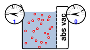
Things get more interesting if we apply equation 6 to seawater just sitting around in an open beaker, subject to 1 bar (absolute) ambient pressure, as shown in figure 13. The blue region represents water, and the red circles represent the solute. The region labeled “abs vac” is absolute vacuum; no solute, no solvent, no nothing.
Mindlessly plugging in the numbers we get:
| (10) |
Obviously there is something not quite right about this; we have left something out of the analysis.
On the seawater side of the membrane, the pressure gauge reads 1 bar (absolute) as it should. On the other side of the membrane, there is no solute and no solvent either. If you put a drop of pure water in there, it would promptly get sucked over to the other side. The gauge on the low-pressure side reads zero pressure (absolute), whereas equation 10 seems to predict -24 bar, so we have some explaining to do.
The first half of the explanation deals with the low-side gauge. The gauge is just an ordinary mechanical gauge. The piston or Bourdon tube (or whatever it uses) can push on the water, but it cannot pull on the water. If the water pressure tried to go negative, the water would just disconnect from the gauge. You can call this cavitation if you wish. It’s hard to make a gauge that reads negative absolute pressure on the scale we’re talking about (although there are always small effects due to surface tension et cetera).
The second half of the explanation deals with the seawater. If the seawater is subjected to a huge negative pressure, why doesn’t it cavitate? Well, for starters, the solute pressure is not really a negative pressure applied to the outside of the liquid; it is a positive pressure applied to the inside of the liquid. This internal pressure i.e. the osmotic pressure i.e. the solute pressure is restrained by the cohesion of the liquid.
And the solute cannot detach from the solvent the way the gauge detached from the solvent. If you have a liquid in a cylinder, and pull out the piston, cavitation allows the piston to move, so that the cylinder volume expands, without stretching the liquid. In contrast, cavitation does not allow the solute to expand, because the solute cannot enter the cavity. The solute doesn’t care about the volume of the cylinder, only about the volume of the solvent.
To repeat: The true solvent pressure should not be considered a negative pressure applied to the outside of the solution. The true solvent pressure does not arise from anything pulling from the outside the solution; it arises from the solute pushing outward from the inside.
In contrast, the so-called solvent pressure in equation 6 and equation 10 is what a gauge (on the outside of the system) reads if/when it is in contact with the solvent. When there is good contact, the gauge force (acting from outside) just balances the solvent pressure (acting from inside) so the equations make sense. When there is not good contact, the solvent pressure is balanced by the cohesion of the liquid, and the equation doesn’t tell us anything about the gauge reading.
The idea of “negative absolute pressure” is not my favorite way of describing the situation, but it does give a correct description of some aspects. This includes the energy budget. You can use equation 6 (and equation 10) without worrying about whether the pressure is negative or not. The P Ṿ energy term does not care whether the pressure is due to a pull from outside or a push from inside. This also includes a broad range of colligative effects, including vapor pressure (reference 4) freezing point (reference 5) et cetera.
Via the P Ṿ term, the solute pressure makes it energetically favorable to expand the volume of the solution – even if the expansion has to suck solvent uphill against a modest gradient in total pressure, as in figure 12.
In a certain unconventional sense, the fact that the solute is trapped in the solvent can be considered a solvation effect. That is, if you measure the energy of the solute relative to its vapor you find that it is energetically favorable for the solute to remain trapped in the solvent. (This stands in contrast to the conventional notion of energy of solvation, which would measure dissolved salt or sugar relative to the corresponding solid, not vapor.)
Cohesion is necessary to balance the force budget, as indicated in figure 14. Let’s consider a parcel of fluid (the large, light-blue rectangle) and analyze the forces on one edge. The solute is represented by the red circles. Solute pressure creates an outward force acting on the surface, as shown by the red arrows. Meanwhile, cohesion in the liquid is represented, metaphorically, by springs in tension. This cohesion produces an inward force acting on the surface.
To summarize:
The idea of “negative” absolute pressure in connection with osmosis is not new. A simple, elegant, and incisive argument can be found in reference 4. For a more modern and more detailed review, see reference 6.
In the case where the solvent is a gas (not a liquid), we never observe a situation where the solution is under tension. There are two reasons for this: there is no cohesion in the solvent, and the solute is not trapped in the solvent.
Here’s an interesting exercise: Put a check-mark in the box next to the best answer. Choose the best way of completing this statement: Other things being equal, for an ideal gas, ...
□ (A) ... when the temperature goes up, the volume goes up, and when the temperature goes down, the volume goes down.
□ (B) ... when the temperature goes up, the volume goes down, and vice versa.
Do you know the answer to that question? I sure don’t. It could go either way ... as you can see by comparing section 1.2 to section 1.3.
We can gain additional insight into this situation by looking at the following figures.
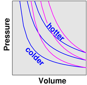
In figure 15, the gas cools as it expands. You can see that if we move left-to-right along a contour of constant entropy, we cross contours of constant T, moving toward lower T values. The contours of constant entropy are steeper than the contours of constant temperature.
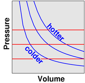
In figure 16, if you want the gas to expand at constant pressure, you have to heat it up. You can see that if we move left-to-right along a contour of constant pressure, we cross contours of constant T, moving toward higher T values. The contours of constant pressure are less steep than the contours of constant temperature.
There is not any law of nature that prefers the isentropic scenario (section 1.3) to the isobaric scenario (section 1.2) or vice versa. Both scenarios can be found in nature, to a good approximation, if you know where to look. Either scenario can be realized in the laboratory, to a good approximation, if you engineer the experiment appropriately.
Some people labor under the impression that since the ideal gas law nicely describes the isobaric scenario (section 1.2), the isentropic scenario (section 1.3) must involve an exception or a breakdown of the ideal gas law. This is completely wrong; the isentropic behavior described in section 1.3 is perfectly consistent with the ideal gas law.
Some people labor under the impression that the isothermal scenario (section 1.4) is “normal”. That’s the result of working slowly, studying only small systems, and not looking very closely: they will never notice much departure from isothermal behavior. In fact, many other behaviors commonly occur, as illustrated by the examples below.
Large-enough systems can be expected to be isentropic, to a good approximation, if the timescale is slow enough to prevent undue frictional dissipation, yet fast enough to prevent undue thermal conduction. Examples abound, including:
Of course, not everything is isentropic:
There is one more technique you need to know to apply the gas laws to things like the atmosphere.
In all the scenarios considered in section 1, the volume V was just the volume of the container. So the question is, what is the relevant V when we are talking about the atmosphere, or any other system where there is no relevant container?
The answer is that we talk about a parcel of gas. That is, take some region of space, and imagine marking all the gas that is initially within that region. We then follow the parcel of marked gas as time goes on. The parcel will move. The parcel will change shape, but that doesn’t matter, except insofar as the volume changes (compressing or expanding the parcel). The boundaries of the parcel might become a bit blurry, as molecules diffuse across the boundary to/from adjacent parcels, but this won’t greatly affect the properties of our parcel, especially if neighboring parcels have approximately the same properties anyway.
The gas laws apply to each parcel of gas separately.
This technique of dividing the overall system into a number of parcels is completely routine in the fluid dynamics business.
Let’s take another look at the exercise mentioned at the beginning of section 3.1. The first few words of the stem should have been a dead giveaway. The words Other Things Being Equal should always make alarm bells ring in your head. I call this the OTBE fallacy. Almost any statement that involves other things being equal is underspecified, because you rarely know which other things are being held equal.
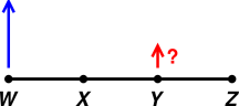
It is easy to explain this to young students. Here’s an analogous exercise: Put a check-mark in the box next to the best answer. Choose the best way of completing this statement: Other things being equal, for the lever in figure 17, ...
□ (A) ... when point W goes up, point Y goes up, and when point W goes down, point Y goes down.
□ (B) ... when point W goes up, point Y goes down, and vice versa.
Do you know the answer to that question? I sure don’t. The answer very much depends on whether point X is the fulcrum or point Z is the fulcrum.
You can make an unforgettable classroom demonstration using a meter stick or suchlike. Attach a bit of tape to point Y to focus attention there. Then choose a pivot-point (X or Z), wiggle point W, and observe what happens to point Y.
This is an example of what we call an ill-posed problem. More specifically, it is underspecified. For a more general discussion of ill-posed problems and how to deal with them, see reference 7.
Returning to the gas laws, we see the crucial importance of keeping track of which variables are being held constant. In particular, P1 V1 = P2 V2 is not by itself law of nature, and by the same token P1 V1(γ) = P2 V2(γ) is not by itself law of nature. The former is valid within the isothermal scenario (section 1.2), while the latter is valid within the isentropic scenario (section 1.3). It would be the most foolish of fallacies to take something that is true only within a particular scenario and pretend it was true more generally.
To say the same thing mathematically, P1 V1 = P2 V2 is merely part of a system of three equations, while P1 V1(γ) = P2 V2(γ) is part of a different system of three equations.
Let’s collect the three-equation systems that appeared in the scenarios discussed in section 1 ... plus a couple of related systems. This is inelegant, but let’s do it anyway:
| (11) | ||||||||||||||||||||||||||||||||||||||||||||||||||||||||||||||||||||||||||||||||||||||||||||||||
If you include the possibility that N could be a variable, the number of systems gets even larger.
Practicing scientists generally don’t remember the gas laws in the form suggested by list 11. That’s because it is far easier to remember just two equations:
| (12) |
This is a win/win situation. These two laws are simpler ... yet also more powerful, more general, more sophisticated, and more elegant than the hodgepodge in list 11. Why be inelegant when being elegant is easier?
Each three-equation system listed in list 11 can be seen as a narrow corollary of equation 12, narrowed by scenario-specific information about what is being held constant. You don’t need to memorize these corollaries, because whenever they are needed, you can re-derive them in less time than it takes to tell about it.
For those who are seriously math-impaired, I will spell out the derivation in lurid detail just once. Let’s take the example of equation 2. How do we get from line 1 to line 2 of that equation?
| (13) |
Of course, someone with a little skill could do the same calculation in far fewer steps; I spelled out the details just to emphasize the point that each step is well-founded in elementary algebra. This is the same sort of algebra that is required for a gajillion other tasks, so you might as well learn it.
The root iso- comes from Greek and means “same”. It is widely used to coin scientific terms, including:
| isobaric | ≡ | at constant pressure | |||
| isothermal | ≡ | at constant temperature | |||
| isochoric | ≡ | at constant volume | |||
| isentropic | ≡ | at constant entropy | |||
| } | ≡ | at constant energy |
The term adiabatic is troublesome. Thoughtful experts use the word in two inequivalent ways:
| α | ≡ | not |
| δια | ≡ | through |
| βατος | ≡ | flow |
I recommend avoiding the term “adiabatic” whenever possible. If you mean isentropic, say isentropic. If you mean thermally insulated, say thermally insulated.
Some textbooks like to give names to a few of the items in list 11. In particular, Boyle’s Law is sometimes mentioned in this context. I have no idea which law goes with that name. Most practicing scientists have no idea, either. They simply remember P V = N kT and P V(γ) = f(S), and that’s all there is to it.
Charles’s Law, Avogadro’s Law, and Gay-Lussac’s Law are also sometimes mentioned, but many practicing scientists have no idea what those refer to; if you told them Gay-Lussac’s law was a corollary of Murphy’s law they might well believe you.
Naming the corollaries to the gas laws is not a terribly big problem; on the scale of things it is trivial compared to the gross misconceptions discussed in section 6. The objections here are pedagogical rather than technical:
The notion of “ideal gas” has the advantage of simplicity, and has rather wide real-world applicability.
However, this simplicity is something of a two-edged sword. Ideal gases should not be over-emphasized, and should not be used as the only example of a thermodynamic system, because many things that are true of ideal gases are not true in general.
For example, in a monatomic perfect gas, all of the heat capacity can be explained in terms of kinetic energy (and changes thereof). This is true for the simple reason that all of the energy is purely kinetic.1 Obviously this isn’t true of all thermodynamic systems, but generation after generation, students somehow pick up the idea that there is such a thing as “thermal energy” distinct from other kinds of energy (which there isn’t), and that the heat capacity of ordinary materials can be explained in terms of microscopic kinetic energy (which it cannot). (For example, the energy associated with the heat capacity of an ordinary solid is very nearly half kinetic energy and half potential energy.)
It is usually a bad idea to discuss misconceptions. That’s because there are always an infinite number of misconceptions, and to discuss even a small fraction of them becomes a horrific waste of time. Usually it is better to describe the right way of doing things, and then move on.
However, an exception can be made for misconceptions that are particularly common and/or particularly destructive.
Sometimes people who ought to know better present the following list to their students
| (14) |
and tell them that in any given scenario, the applicable equation can be selected using the “principle” that the variables not mentioned are being held constant. For example, the first line in list 14 doesn’t mention N or V, so allegedly those variables “must” be considered constant. That is, alas, completely bogus. The first line doesn’t mention number, volume, entropy, enthalpy, free energy, free enthalpy, and/or innumerably many other variables that might be relevant in this-or-that scenario. If you know which variables are being held constant, and look down this list to find an equation that doesn’t mention them, you will almost certainly find an equation that is not applicable.
The just-mentioned procedure has absolutely no basis in physics, mathematics, or logic.
The only way such a procedure can even appear to work is in the fairy-land situation where the person asking the questions and the person answering the questions are both so clueless that they are unaware of scenarios where variables other than N, V, P, and/or T are held constant.
The fundamental problem is that none of the equations in list 14 is, by itself, a law of nature. There are only two ways to repair this situation.
To say the same thing more formally, each equation in list 14 is merely part of a system of three equations ... a different system in each case. You have to learn each system as a whole, which takes us back to a subset of list 11. It is permissible to choose an appropriate line from list 11 ... based not on which variables are missing, but rather on which variables are explicitly held constant by equations on the chosen line.