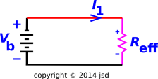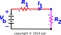
Figure 1: Resistors in Series : Voltage-Divider Circuit
Kirchhoff’s Circuit «Laws» provide a simple approximate description of how voltage and current behave in electric circuits. People really like this simple way of looking at things, and they often take pains to design their circuits so as to minimize the importance of the various violations of Kirchhoff’s «laws». However, the direct usefulness of these «laws» is far less than you might have imagined. The range of useful applicability gets squeezed from above and from below:
When in doubt, rely on the Maxwell equations, not Kirchhoff’s so-called «laws».
Kirchhoff’s Voltage «Law» (KVL) – aka Kirchhoff’s Loop «Law» – alleges that the voltage around any closed loop is zero. There are some very serious limitations to the validity of this «law», as discussed in section 1.5. First, though, let’s figure out what this «law» tells us, in a best-case scenario.
Let’s apply KVL to the circuit in figure 1.
You might want to review basic concepts of voltage, as set forth in reference 1. Voltage is defined with respect to a path. Let’s choose a path, namely a closed loop that goes clockwise, following the wires and circuit elements. Then KVL alleges that
| (1) |
That’s OK for a start, but we can obtain additional information by considering additional paths. Let’s consider three separate sub-paths and the associated voltages, namely:
These three contributions add up to make the whole loop. So if we are careful about the orientations, we can write
When applying equation 2a, we need to keep the various ΔV contributions properly oriented. The rule is to go around the loop in a particular direction, adding up the voltage increases. A positive ΔV represents a voltage increase.
Narrowly speaking, that is as far as we can get using KVL alone. However, we can make additional progress if we bring in Ohm’s law. For each resistor:
| (3) |
Ohm’s law tells us there is a voltage drop associated with each resistor. This assumes we have chosen directions consistently, so that the nominal direction of the current I is the same as the forward direction along the path we are using to define the voltage. A voltage drop corresponds to a negative ΔV. For details on the sign conventions, see note 1.
If you have trouble keeping track of what’s a voltage drop and what’s a positive ΔV, you can pencil in little positive and negative signs next to each resistor, as we have done in figure 1. With a little experience, this step becomes unnecessary.
Combining Ohm’s law with KVL gives us:
We can reformulate Kirchhoff’s voltage «law» as follows: Pick any two points in the circuit (A and B). We suppose there are two or more ways of getting from A to B, and we call these the legs of the circuit. Then Kirchhoff’s voltage «law» says that the voltage increase in each leg is the same.
Let’s apply this to figure 1. We choose point A to be the southeast corner of the circuit, and point B to be the northwest corner. There is a black leg (containing the battery) and a colored leg (containing the two resistors in series). Applying this to the circuit in figure 1 we find:
We have obtained this directly by comparing legs. (We could also have obtained it by rewriting equation 4b.)
Real-world electrical engineers are very fond of the leg-by-leg approach. This is probably because with the loop-by-loop approach, when there are multiple loops, it can be annoying to keep track of how the loops mesh together. In contrast, it is straightforward to keep track of the relationships between all the various legs.
| When φ•=0, the leg-by-leg approach is completely equivalent to the loop approach. Anything you can calculate one way you can calculate the other way. You should verify this for yourself. | When φ•≠0, the leg-by-leg approach gives a more detailed picture of what’s going on. It’s more work, but it’s more informative. |
Also, a reminder: As discussed in section 1.1, there is a voltage drop as we go along the colored path in the direction of the current I. By the same token, there is a positive ΔV if we go along the path in the other direction, from point A to point B. All this is predicated on I corresponding to positive current flowing in the direction indicated by the arrowhead on the diagram.
Now that we know the current I1 we can apply Ohm’s law to find the voltage drop across R2, namely
|
Combining this with previous results, we obtain
|
To say the same thing in words: Given a string of resistors in series, the voltage drop across one given resistor is to the total voltage drop as the resistance of the given resistor is to the total resistance. This is called the voltage-divider rule. It is very widely useful.
Starting from equation 5, we can apply Ohm’s law in reverse to discover that the series combination of resistors that we see in figure 1 presents the same load as a single resistor with value
| (8) |
Figure 2 shows the so-called equivalent circuit. It must be emphasized that this is equivalent only as far as the battery is concerned. That is to say, it presents an equivalent load on the battery.
Equation 8 is the rule for resistors in series. It generalizes to any number of resistors, from one on up. It says that for resistors in series, just add up all the resistances.
This is important, because in the real world, engineers seldom invoke KVL directly. Instead, they apply things like equation 8. This has the advantage of being somewhat simpler and more convenient. This equation is of course a corollary of KVL, and suffers from all the limitations as KVL itself, as discussed in section 1.5.
This is the bread and butter of circuit analysis: Replacing a complicated circuit by a simpler equivalent circuit.
There are some very serious limitations on the validity of Kirchhoff’s voltage «law», as we now discuss.
It is sometimes quite tricky to decide what’s significant and what’s not.
On the other hand, in the real world, this is not something you can take for granted. If you want KVL to be a good approximation, you have to arrange for it by means of suitable engineering. Sometimes it is not even possible, especially when dealing with high-power, high-precision, and/or high-frequency circuits.
In situations where KVL does not apply, it’s not the end of the world. You have to analyze things in more fundamental terms. In particular, if there’s ever a conflict between Kirchhoff’s «laws» and the Maxwell equations, go with Maxwell.
We can understand the origins of Kirchhoff’s voltage «law» – and its limitations – in terms of Faraday’s law of induction, which is one of the Maxwell equations. It can be written in many forms, of which the following most directly serves our purposes:
| (9) |
This is pronounced “voltage equals flux dot”. The LHS is the voltage drop around a closed loop, and the RHS is the rate-of-change of the amount of magnetic flux threading the loop. In more detail:
| (10) |
so we can restate equation 9 as:
| (11) |
where E is the electric field, B is the magnetic field, S is some patch of surface, the loop ∂S is the boundary-curve of that surface, ds is the element of arc length along the boundary, and dA is the element of area on the surface. This fundamental law applies to any loop you can think of. Typically the loop is defined by wires and circuit elements, but this is absolutely not required. It also applies to any surface you can think of, so long as ∂S is the boundary of S.
If the voltage is a potential, then the loop voltage will be zero, as called for by Kirchhoff’s «law». However, as discussed in reference 1, non-potential voltages are often desirable ... and are often present whether they are desired or not.
Procedures for designing circuitry to minimize the effects of KVL violations – and for measuring violations when they do occur – are discussed in reference 2.
Kirchhoff’s Current «Law» – aka Kirchhoff’s Node «Law» – states that if N current-carrying wires meet at a node, the sum of the currents must be zero. Inbound currents count as positive, and outbound currents count as negative. There are very serious limitations to the validity of this «law», but first let’s see what this law tells us in a best-case scenario.
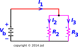
Let’s apply KCL to the node represented by the black dot in figure 3.
KCL tells us the that total current into the node is:
| (12) |
We can also interpret this in terms of current in and current out. The incoming current is I1. The total outgoing current is I2 + I3. The outgoing current is carried by a parallel combination of resistors, namely R2 in parallel with R3.
| (13) |
We can combine equation 13 with Ohm’s law to find
| (14) |
Consider the following two points:
Both of these assumptions are necessary in order to make KCL meaningful. They are very often taken for granted. This is a problem, because both of them have seriously limited validity.
Let’s lump these two assumptions together and call them Kirchhoff’s Third «Law» (K3L). We consider that KCL requires K3L, and therefore any violation of K3L is counted as a violation of KCL also.
We can find the current in one leg of the circuit as follows:
|
To say the same thing in words: Whenever there is a bunch of resistors in parallel, the current in one given resistor is to the total current as the inverse resistance of the given resistor is to the total inverse resistance. This is called the current-divider rule. It is very widely useful.
The inverse resistance is called the conductance and is denoted G. So we can rewrite equation 15 as:
| (16) |
You can see that this is the mirror image of the voltage divider law, equation 7.
Starting from equation 13, we can apply Ohm’s law in reverse to find that the combination of resistors in figure 3 presents the same load to the battery as a single resistor with value
| (17) |
We can write this in more symmetrical form as
| (18) |
We can also define a new mathematical operator such that
| (19) |
This ∥ operator has a number of remarkable properties, including associative, commutative, and distributive properties, as discussed in reference 3.
| (20) |
Figure 4 shows the so-called equivalent circuit. This is identical to Figure 2. It must be emphasized that this is equivalent only as far as the battery is concerned. That is to say, it presents an equivalent load on the battery.
This is important, because in the real world, engineers seldom invoke KCL directly. Instead, they apply things like equation 17. This has the advantage of being somewhat simpler and more convenient. This equation is of course a corollary of KCL, and suffers from all the limitations as KCL itself, as discussed in section 2.5.
There are some very serious limitations on the validity of Kirchhoff’s current «law», as we now discuss.
For example, suppose node A carries a high-voltage AC signal, and suppose node B is a sensitive, high impedance, low voltage receiver circuit. Any appreciable parasitic capacitance linking those two nodes would be intolerable. There are many things we can do to alleviate the problem:
The outer conductor on a coaxial cable is an example of the kind of shielding we’re talking about. Think about it:
The point is, without shielding, there would be widespread gross violations of KCL.
In the real world, KCL cannot be taken for granted. If you want KCL to be a good approximation, you have to arrange for it by means of suitable engineering. Sometimes it is not even possible, especially when dealing with high-power, high-precision, and/or high-frequency circuits.
In situations where KCL does not apply, it’s not the end of the world. You just have to analyze things in more fundamental terms. In particular, if there’s ever a conflict between Kirchhoff’s «laws» and the Maxwell equations, go with Maxwell.
We can understand the origins of Kirchhoff’s current «law» – and its limitations – in terms of conservation of charge, which is implied by the Maxwell equations.
In the low-frequency limit, we can make the following argument: We assume the size of the node is finite, therefore the self-capacitance of the node is finite. We further assume the voltage on the node is finite. Combining those two ideas, the charge on the node must be finite. current is charge per unit time, and the timescale is very long, so the current must be very small. Therefore KCL is valid to a good approximation.
In AC circuits, KCL sometimes fails. Significant violations of KCL can occur even at 60 Hz, which is not a very high frequency. For a spectacular example of this, see the video in reference 4. If you consider the helicopter to be a node, unbalanced current is flowing into the node and back out again, at a frequency of 60 Hz.
On a smaller scale, a very helpful violation of KCL is the basis for a non-contact voltage detector. The detector is not connected to the circuit by any conductors. There is also not any need to connect the detector to ground; all it needs is a large-enough self-capacitance, like the aformentioned helicopter. The detector is an isolated node. If there is a nearby wire or other object carrying an AC voltage, the alternating electric field will give rise to some charge flowing to and from the detector node, and this can be measured. See reference 5.
Indeed, in practice, most of the problems with KCL are associated with parasitic mutual capacitances.
You are encouraged to skip this section, especially on first reading. The main purpose is to dispel various specific misconceptions. If you do not suffer from any of these misconceptions, that’s good, and you should not waste brain cells thinking about them.
Ohm’s law is usually written as an expression for the voltage drop, as in equation 3. We speak of the IR drop. A drop corresponds to a negative ΔV if you go along the path in the direction of the current I.
I mention this because some people write
| (21) |
which is wrong by a factor of −1, or at best inconsistent with near-universal conventions as to what “Δ” means. It is much better to write Ohm’s law in terms of the voltage drop, as in equation 3.
| If you encounter a circuit that is working properly, it is quite likely that Kirchhoff’s «laws» apply to this circuit, to a reasonable approximation. | If you encounter a circuit that is not working properly, there is a good chance that Kirchhoff’s «laws» are being violated. |
In particular, when faced with excessive hum or noise or interference, you should consider all the possible nonidealities that could be causing the problem. High on the list is the possibility that a KVL violation could be injecting some unwanted voltage into some leg(s) of the circuit.
Note that at the beginning Kirchhoff’s «laws» are assumed valid, and at the end they are actually valid. However, one must not neglect the crucial middle stage, where Kirchhoff’s «laws» are not valid. If the engineer understands why, where, and how much Kirchhoff’s «laws» are being violated, he will have a much easier time getting past the middle stage.
Either KVL or KCL separately is sometimes called simply Kirchhoff’s «law». The meaning is usually obvious from context.
The goal of this section is to understand the voltages and currents in the mesh circuit shown in figure 6. However, before we get to that, let’s do a simple warm-up exercise.
Specifically, let’s start by considering the simple circuit shown in figure 5. There is a square loop made of resistors. All four resistors have the same value, namely R. There is an applied magnetic field perpendicular to the plane of the circuit. The magnetic field is uniform in space. The relevant component of the magnetic field is steadily increasing. In accordance with Faraday’s law of induction, this induces an electric field. The electric field is everywhere parallel to the plane of the mesh. Roughly speaking, the electric field points in a direction specified by the three blue arrows surrounding the φ• symbol. This field is not the gradient of any potential. The total voltage around the square loop is V0. The voltage drop across each resistor is V0/4. The current in each resistor is I0/4, where the “reference current” is I0 := V0/R. This represents a steady current, an induced current, flowing around the loop. We imagine that the resistance is small, so the induced current is enormous.
We integrate the magnetic field over the area of the square. This gives us the magnetic flux, φ. The rate-of-change is constant, namely φ•. Faraday’s law of induction tells us that the voltage drop around the square is V0 = φ•.
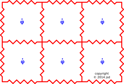
We are now ready to analyze the mesh circuit shown in figure 6. There are six square cells, all with the same area. Each cell is bounded by four resistors. Each of the 17 resistors has the same resistance, namely R. Roughly speaking, the electric field in this case is the superposition of six copies of the field we saw in figure 5, but in some places the contributions add or cancel. Finding the details of the electric field would be more work than necessary, because all we really need to know is the current in the wires and the voltage measured along the wires. However, we do know one thing already: The electric field determines the voltage around each loop, in accordance with the definition of voltage. For each small square loop, the voltage is V0.
We consider the following quasi-steady state: The magnetic field is not steady, but rather the derivative ∂B/∂t is steady. The electric field is steady. Any initial transients have died out, so all the voltages and currents in the circuit are steady. The flux φ is the same from cell to cell and also φ• is the same from cell to cell. The voltage around each small square cell is V0 = φ•.
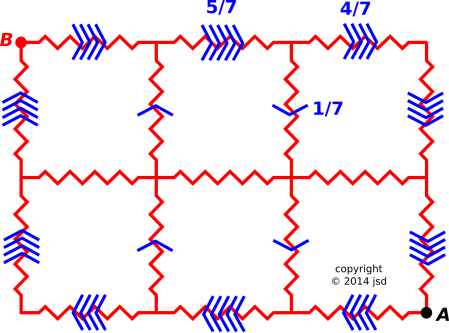
For the six-cell circuit, it is a bit of work to find all the voltages and currents. On the other hand, given the solution shown in figure 7, it is not hard to verify that the solution is correct. In the figure, each blue arrowhead represents I0/7, i.e. one seventh of the reference current. If you multiply this by R, you find that each blue arrowhead counts for one seventh of the induced voltage in each cell.
You should check that on the boundary of each cell the net number of clockwise-pointing blue arrowheads is seven. This means that the solution upholds Faraday’s law of induction, in agreement with the amount of φ• specified in figure 6. You should also verify that the net current into each node is zero, in accordance with Kirchhoff’s current «law». You should also verify that everything we have said about the current/voltage relationship is in agreement with Ohm’s law.
Note that all of these voltages are non-potential voltages. They are perfectly well defined if you talk about the voltage along a path, but you get nonsense if you try to talk about “the” voltage at a point. For example, consider the resistor that proceeds rightward from point B. I can tell you absolutely that the voltage drop across this resistor is 4/7ths of V0. I cannot tell you “the” voltage at either end of this resistor, not even approximately, but I can tell you the ΔV quite accurately.
Here’s another look at why the voltage must be a functional of the path, not a function of position:
| Consider the clockwise path from point A to point B, running along the bottom and the left side of the diagram. There is a drop of 21/7ths i.e. 3 units of voltage along this path. | Consider the counterclockwise path from point A to point B, running along the right side and the top of the diagram. There is a gain of 21/7ths i.e. 3 units of voltage along this path. |
Now obviously, you cannot have a voltage at point B that is simultaneously less than and greater than the voltage at point A.
Note that Kirchhoff’s voltage «law» implies that the voltage is a potential. KVL cannot possibly give the right answer when applied to this circuit. Faraday’s law of induction gives the right answer, but KVL does not.
Also note that you cannot “salvage” KVL by rebuilding the circuit using different components. In particular, so far as I know, you cannot set up the pattern of currents and voltages shown in figure 7 using any combination of batteries, resistors, wires, and other lumped-circuit elements. That’s because the lumped-circuit model would guarantee that the voltage would be a potential. It would uphold KVL, whereas the actual circuit does not. Let’s be clear: KVL says that every time you connect a battery and a resistor, there is some voltage drop in the resistor along with (roughly) an equal-sized voltage gain in the battery. The situation in figure 7 is wildly different: There are voltage drops (i.e. IR drops) associated with each of the resistors, but there are no batteries!
Motivation: There are several non-ridiculous ways in which a circuit like this could come to exist. For one thing, suppose there is a large time-dependent magnetic field, and you want to screen it, so that it does not cause horrible interference with all the electronics in the neighborhood. You might well model the screen in terms of a mesh. This could be on a smallish scale (such as the ground plane of a circuit board) or it could be very much larger.
Also, imagine you’re a farmer. There is a lot of metal mesh on the floor of your dairy barn. There is some old, clunky yet powerful equipment that puts out a large time-varying magnetic field. You suspect that this is inducing enormous currents in the mesh. You have made several valiant attempts to measure the voltages and currents, but you keep getting inconsistent results ... reproducibly inconsistent!