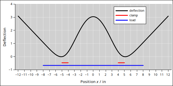
Figure 1: Deflection of a Loaded Beam
Suppose you wanted to glue a thin strip of wood to the front edge of a shelf, to make it look nicer. The conceptually simplest approach would be to apply glue and clamp everything until the glue sets. However, that would require a great many clamps, because the strip is long, thin, and flexible.
The best approach would be to use jig, namely a long, straight, and very strong spreader to push on the thin strip. Then apply clamps to the other side of the spreader.
Now suppose the only thing you have to serve as a spreader is long enough and straight enough, but slightly flexible. You can put shims between the spreader and the strip to account for the flex, so you wind up with a uniform distribution of force.
It would be nice if we can calculate in advance the thickness of the shims requires. In some sense this “should” be easy, using Green function methods. However, simply turning the crank, applying the method without thinking, results in an ugly mess; you wind up with a Green function that doesn’t satisfy the boundary conditions.
If you try googling for the answer, you get all sorts of results that are worse than useless. You can easily find expressions for G when the beam is clamped at one or both ends. You can also find long, messy studies of the dynamics of a beam with free ends and unbalanced forces.
The fundamental problem is that there does not exist a static solution for the deflection that results from a delta-distribution of force. So in some sense equation 1, which defines the Green function (G) for our situation, is unphysical.
| (1) |
where δ is the Dirac delta.
Homework: Turn the crank on equation 1. That is, integrate it four times to find G. Then try to satisfy the boundary conditions. This is guaranteed to fail, but it’s interesting to see why it fails. This is not wasted effort, because the calculation can be re-used in what comes next.
Using clamps in the usual way, we have a static situation with a balanced distribution of forces. Furthermore, we can arrange the clamps so that the forces are symmetrical about the center, which simplifies the calculation.
Our task, therefore, is to find a Green-like function that embodies the physics of the situation. So let’s consder a combination of forces, namely force applied at point z, together with other forces to provide balance. That adds up to:
| (2) |
where the symbol ≐ is meant to represent equilibrium. The superscript is a reminder that this is a balanced distribution of forces. This is manifestly an even function of z, we have nothing to lose by assuming z≥0. This allows us to use terms like “right” and “left” in the discussion that follows. It is also relevant to equation 12.
The Euler-Bernoulli equation for small deflections of a loaded beam is:
| (3) |
where w is the deflection, F is the applied force, E is the elastic modulus, and I is the second moment of are of the cross-section of the beam (which may depend on x). The product EI is known as the flexural rigidity. See reference 1 for the next level of detail on this.
In the situation of interest, the beam is uniform; that is, EI is independent of x. So the equation simplifies to:
| (4) |
We have already done the hard part, which is to realize that we need to base our calculation on a balanced distribution of forces. The next step is to integrate equation 2 four times, which is straightforward. Then we have to account for the boundary conditions. In our application, the boundary condition is free ends.
We will make use of the step functions:
| (5) |
Mnemonic: Look at the shape of the letters L and J. Their derivatives are:
| (6) |
The integrals are:
| (7) |
| (8) |
| (9) |
| (10) |
We can expand the last equation as:
| (11) |
From here on, we treate є as zero.
Note that if we had kept only the first two terms on the RHS of equation 2 (i.e. dropping the “near” terms), we would have wound up with a term in +x3 on the right and −x3 on the left. We could have used the C1x3/6 term to cancel one or the other but not both. We need to cancel them, because the free ends are straight. Keeping all four force terms, there is a nice cancellation in the far left and right regimes. We conclude C1 must be zero (which should have been obvious from symmetry).
Also by symmetry, C3 must be zero.
In the far zone, both left and right, there is a term −3zx2/6. We need to get rid of that, so we choose C2 = z.
Finally, we choose C4 = 0, so that in the near zone, both left and right, the constant term is 0. The means the Green function goes through the point (0, 0).
Putting this all together, we have:
| (12) |
Recall that z≥0, so we can freely substitute |z| for z and vice versa. This allows equation 12 be rewritten in the elegant form:
| (13) |
where x< is the smaller of {x, z} and x> is the larger. This makes the symmetry of the Green function manifest. Among other things, this makes it extra-obvious that the near-zone displacement is equal to the far-zone displacement when x is equal to z. (Writing things in terms of x< and x> is very common in the Green function business.)
Note that the last two terms in equation 2, i.e. the “є” terms, drop out when we integrate to find the actual deflection, integrating over a balanced distribution of forces:
| (14) |
So in some sense we have done more work than necessary; it is obviously necessary for w and F to have the correct symmetry, but we have taken the extra step of creating a G≐ that has the correct symmetry all by itself.
Figure 1 show the result of our calculation. The blue trace shows the force due to the load, i.e. the force on the strip pushing up on the spreader, which is 16 inches long. The red traces indicate the downward force applied by the clamps, each of which is 1 inch wide. The black trace shows the deflection of the spreader. Roughly speaking, the shim needs to be 3 units thick in the middle, 2 units thick when x is ± 2 in, and 1 unit thick when x is ± 3 or ± 8 in.