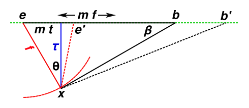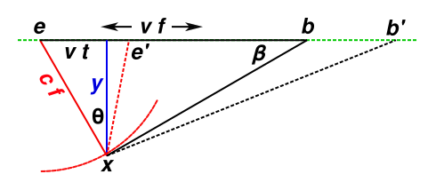
Figure 1: Mach Angle Construction
We consider the times and angles you perceive when a source changes position faster than the speed of sound. The same analysis applies when a source changes position faster than the speed of light, which actually can happen, as discussed below.
| (1) |
The time t is measured relative to the point of closest approach, so for the situation shown in the diagram, t is less than zero.
| (2) |
| (3) |
See also the scaled versions in section 5.
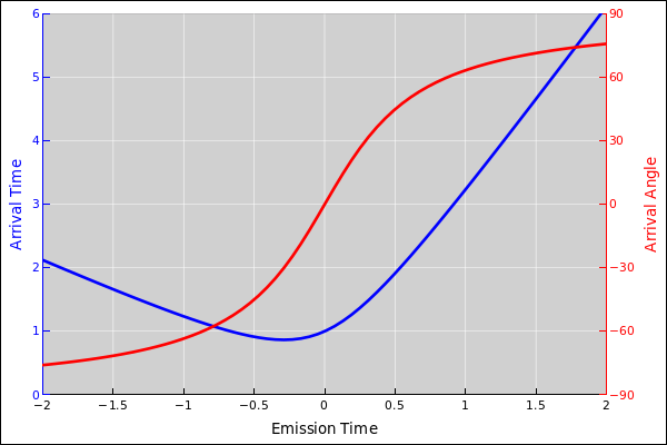
It is now straightforward to solve for the arrival time a and angle θ (both which you can observe directly) as functions of emission time t (which you can’t). The results are shown in figure 2. For this example, we assume y=1, c=1, and v=2.
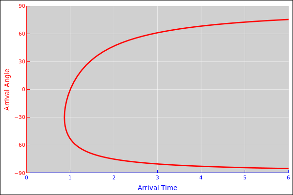
Here’s the graph of what you actually observe: Arrival angles as functions of arrival time. For each time there are two angles.
When there are two signals arriving at the same time, it is tricky to perceive the angle of either of them using just your two ears. It may be possible to untangle them using frequency information, due to the Doppler shift and/or dispersion. You could easily untangle them using a phased-array passive sonar receiver.
Things are even more interesting when you look at a source that changes its position faster than the speed of light. Your eyes contain millions of photoreceptors, so it is possible to perceive both of the arriving signals. You can’t have a source that physically moves faster than the speed of light, but you can have a long array of sub-sources that light up in turn, by pre-arrangement, creating a pattern that moves faster than the speed of light. As a particularly simple example, you can use to grids to create a moireé pattern that moves faster than the speed of light, even though neither grid is moving very fast, as shown in figure 4.
At the time of onset, when the first signal arrives, [e x b] is a right triangle, and β = θ. We know it’s a right triangle because the line [x b] is tangent to the wavefront, as suggested by the circular arc in the diagram. This can be used as a check on other ways of calculating the minimum time of flight f. Also it tells us that
| (4) |
which is the famous formula for the Mach angle.
Also, the emission time of the onset signal is:
| (5) |
In the special case where v/c = 2, at onset the triangle [e x b] is a 30-60-90 triangle. This is the case shown in the diagram.
At some later time, we might be tempted to consider the triangle [e′ x b′], but (1) it doesn’t tell us anything we don’t already know, (2) it bears no relationship to the physics of the Mach angle, and (3) it is not a right triangle.
It is good practice to thing about how a problem scales. For the Mach arrivals problem, all the speeds scale in proportion to c, and all the times scale in proportion to y/c. If we replace v/c by m (the Mach number) and replace y/c by τ (the time of flight from the point of closest approach), then c drops out of the equations entirely. This reduces the number of variables involved. All the legs in figure 5 have dimensions of time (not distance).
The key equations become:
| (6) |
| (7) |