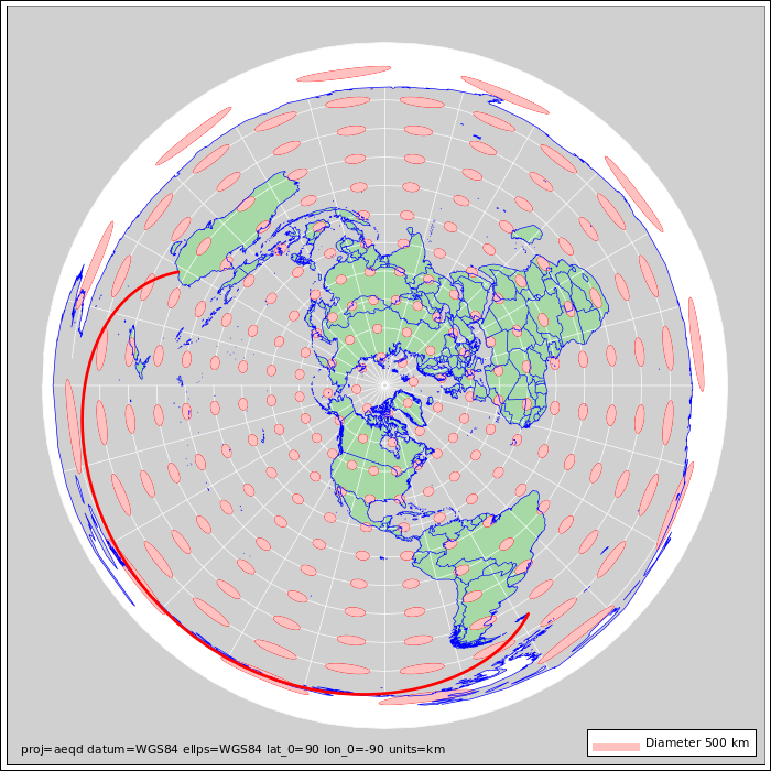
Figure 1: Azimuthal Equidistant Projection : Earth
Here’s a good way describe and quantify the flatness of a flat space, or the curvature of a curved space.
The first step is to figure out the metric of the space.
For example, you may have learned in high school that in a flat plane the distance (ds) can be expressed in Cartesian coordinates as:
| (1) |
We can describe the same flat plane in polar coordinates, in which case the metric is:
| (2) |
where ρ is the radial distance from the origin, and λ is the azimuthal angle, measured in radians. It is more elegant to have both the radial and azimuthal coordinates be dimensionless, so we can treat them on the same footing. So we can write ρ = X θ, where the range θ is dimensionless, and X is some overall scale factor, with dimensions of distance per unit angle. Then the metric becomes:
| (3) |
All of the above are provably flat-space metrics, as discussed below.
On the surface of a sphere, the metric is
| (4) |
where λ is the longitude and θ is the colatitude, both measured in radians. The colatitude goes from zero at the north pole to 180∘ (i.e. π radians) at the south pole. The scale factor X is the radius of the sphere.
Note that equation 4 is very similar to equation 3. Just substitute sin(θ) for θ in one place.
Any map that is a legit projection of a sphere must agree with equation 4. That makes sense, because the equation is expressed in terms of miles per degree.
Meanwhile, different projections differ in the way the represent each degree. For example, on a basic Mercator projection there is a constant number of degrees per inch in the E/W direciton, whereas on a azimuthal equidistant projection (as in section 4.1) the E/W degrees per inch is strongly dependent on distance from the center.
The metric for an ellipsoid is slightly more complicated than for a sphere, but only slightly, and we don’t need to worry about it right now.
Suppose you know the metric as a function of position. Then it is straightforward to calculate the intrinsic curvature of the space that the map represents, as set forth in reference 1. Laborious, but straightforward.
I recommend doing the calculation using a computer-algebra system. The cadabra2 system makes this particularly easy. See reference 2.
The calculation of curvature applies not just to real-world spaces, but also to maps that represent the spaces. It applies even if the maps are imperfect, provided the scale factors are known accurately.
Let’s be clear: Even if the map is made of flat paper, the scale factor (i.e. the metric) will tell you the curvature of the real-world space that the map represents. For example, start with a sphere. Then project it onto a flat map using an azimuthal equidistant projection. The scale of the map in the east/west direction, i.e. the miles per inch, will be vary drastically as a function of position. When you take that into account, you find that the miles per degree agrees with equation 4, as it must.
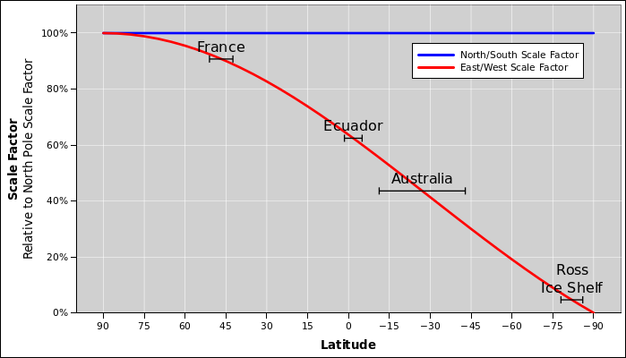
Figure 1 shows an azimuthal equidistant projection. At high northern latitudes it’s not too bad (although you can do better). As you go farther south it gets worse and worse.
The North/South scale factor is uniform everywhere on the map, which is great but it’s not the whole story. As shown in figure 2, East/West scale factor is off by 60% at the equator, and off by a factor of 2.3 by the time you get to Australia. It’s off by a factor of infinity at the south pole.
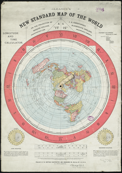
The infamous Gleason map is shown in figure 3. If you ignore the scale bars, it looks like an azimuthal equidistant projection of the real world, with all the same properties set forth in section 4.1.
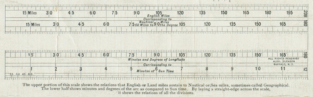
However, when we take into account the scale bar at the bottom of the map, things get ugly. Gleason intended it to serve as proof that the earth is flat, and flat-earthers have used it as such for more than 100 years.
It’s not entirely clear how the scale bar should be used, but it strongly suggests that the map has a uniform scale, in miles per inch, because there is only one scale and nothing is said to limit the places and directions where it applies. Certainly there is nothing that comes anywhere close to setting forth the sin(θ)/θ dependence that would be needed before you could use the map as a representation of the real world.
A uniform scale means the map does not represent the real world. It represents a fantasy land, a flat land in which Australia is more than twice as large east/west as it is north/south.
Here’s a way to quantify the damage done by the bogus scale bars: Any map is, of course, a one-to-one representation of itself. One inch of map per inch of map. The metric for distances on the page is given by equation 3. It’s as flat as flat can be.
Now, as soon as you say that the scale of the map is the same everywhere, i.e. the same number of miles per inch, then the space it represents has a metric of the same form, namely equation 3, just with a larger X factor. So the space is provably flat.
The Gleason map is provably not a representation of the real world, because the shapes on the map do not correspond to shapes in the real world, except perhaps at high northern latitudes.
Hypothetically, if you gave the Gleason map a different legend and different scale bars, you could perhaps transform it into a legit projection of the real world; not a very convenient projection, but still a legit projection. That would leave the graphics unchanged, but would greatly change its meaning.
As it stands, it’s not a projection at all, because of the bogus scale bars.
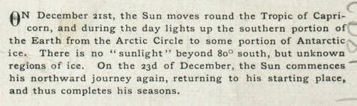
Additional flat-earther nonsense can be seen in the “Capricorn” paragraph near the lower-right corner of the map. In 1892 it was true that the south pole was “unknown” in the sense that nobody had been there. Even so, 50 years earlier the James Clark Ross expedition had sailed within a couple hundred miles of 80∘ south, so the claim that there was “no sunlight” there in December was absurd. Gleason is defying the facts on this point.
Also, the southernmost parts of the map are based on the records of nsuch expeditions. The measured real-world distances are a factor of 10 less than what the Gleason map shows. Also the shapes are categorically different. So he is defying the known facts on these points also.