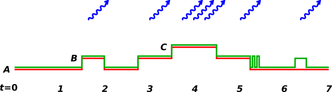
Figure 1: HMM States and Transitions
This document is meant to be a conversation-starter. In particular, I wanted to gather up some diagrams and some terminology in order to make discussions proceed more smoothly. There are few if any conclusions here. Mostly I am just thinking out loud.
In order to explain how a Hidden Markov Model (HMM) might apply to photon timestamping, let’s construct a simplified model using three states, as shown in figure 1.
We assign physical meaning to each state, as follows:
In our simplified model, we ignore the possibility of multiple particles in the detection volume, and ignore lots of other messy details. The topology of the apparatus tells us that direct AC and CA transitions are disallowed (although the HMM formalism could certainly handle such transitions if desired).
Each state is a Poisson process that emits photons at some rate, denoted RA, RB, and RC. We imagine that RC ≫ RB ≫ RA, and that RA is small but not quite zero.
Each transition occurs with some probability per unit time, denoted PAB, PBA, PBC, and PCB. Each such probability is a function of the time t′ that the system has been in its current state.
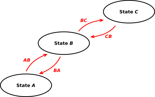
We can draw a timeline of the state of the model, as shown by the red curve (or the green curve) in figure 2. We compare this with the actual data, as shown by the blue “photon” symbols at the top of the figure.
We see that either curve is reasonably consistent with the data, insofar as there are a lot of photons emitted per unit time when the model is in state C and far fewer when the model is in state A.
Roughly speaking, we can fit the model to the data by:
We adjust the parameters as follows: We construct an objective function which measures the inconsistency between the model and the data ... and then tune every parameter in sight to minimize the objective function. Typically the objective function quantifies the “log improbability” log(1/P) or something similar.
For starters, consider each instance of state C in the timeline. Given the time-duration of this instance, and given the Poisson parameter RC, we can calculate a Poisson distribution. We can calculate the likelihood that the distribution could produce the number of photons we see in the data during that time-interval. We include the log-improbability as one term in the objective function.
Tangential remark: Note that least-squares fitting can be thought of as belonging to the same category of optimization procedures, in the sense that the squared residual (with an appropriate weighting factor) is exactly the log improbability, if you think the data is Gaussian distributed. Hint:
−log(exp
−(x−µ)2 2σ2 ) =
(x−µ)2 2σ2 −log(Gaussian) = weighted squared residual (1)
Here, though, we think the time-series data is locally Poisson distributed. That means (among other things) that we don’t need a separate weighting factor. Whereas Gaussians are a two-parameter family of distributions (mean and standard deviation), Poissonians are a one-parmeter family of distributions. If you know the Poisson parameter RC, you know where the peak of the distribution is and you know everything else, including the effective width of the distribution. Although the question of “how do we weight the data” is ultra-important in other contexts, it should never come up in this context.
We can also build other types of knowledge about the physics into the model. For one thing, the physics of diffusion determines how PAB and PBA depend on t′. Suppose the previous state was A, and we have been in state B for only as short time, so t′ is small. Then we expect the transition probability PBA to be quite high, on the order of 50%, because the particle can random walk back and forth over the boundary. An example of this is seen near time 5.3 in the green curve in figure 2. On the other side of the same coin: in this scenario, we expect PBC to be zero at t′=0, because the particle cannot diffuse very far in a short amount of time.
Remark: At this point we have a second-order Markov model, because the transition probability (at short times) depends on both the current state and the previous state. This should not pose any serious difficulties.
When t′ is large, we expect the transition probabilities to be independent of time, and independent of how we got into the current state.
The Baum-Welch “forward-backward” algorithm is a widely-used scheme for optimizing the parameters of the model. I haven’t looked at this recently, but I seem to remember that the generic version of this algorithm assumes that the objective function is a differentiable function of the parameters. Alas, our raw data is basically a bunch of delta functions and the model is a bunch of step functions, so the fine structure of the objective function will be quite gnarly. This may require tweaking the search algorithm used for the optimization. This sounds like work, but it is doable.
| The red curve in figure 2 is a path. The green curve is another path. The probability of the data depends on the sum of probabilities, summed over paths. | In this business, some people habitually assume that the sum is dominated by its largest term (i.e. the “winning path”). This is the basis for treating the problem as an optimization. Examples include least squares algorithms, Viterbi algorithms, et cetera. |
| Sometimes it is very important to consider multiple contributions to the sum. | Sometimes the sum really is dominated by its largest term, to a satisfactory approximation. |
Note that we have a sum of products: As we go along a path, we add the log improbabilities, which is tantamount to multiplying probabilities. Then we sum over paths, summing the actual probabilities (not the log improbabilities).
For example, in figure 2 the green curve is slightly less probable than the red path, because of the blip at time 6.3. This blip does a better job of explaining the data, but the occurrence of the blip is a priori improbable. In any case, if you remove this blip the green curve should have very nearly the same probability as the red curve, and both curves (along with many others) will contribute to the sum.
You can think of the probability calculation as a path integral of the sort that occurs in quantum mechanics (reference 1). More precisely, it is the same sort of path integral that occurs in thermodynamics, since we are adding real probabilities rather than complex probability amplitudes. (In this way, thermodynamics can be considered the analytic continuation of quantum mechanics and vice versa. Steepest descent versus stationary phase.)
It’s relatively easy to create a training procedure that trains the model to calculate the probability of the data given the model.
However, what we almost certainly want is the reverse, namely the probability of the model given the data. It takes some cleverness to devise a training scheme to do this, but it can be done.
The whole point of the exercise is to learn something about the physics.
We want to build the model in such a way that the parameters of the model – RC, RB, PAB, et cetera – speak to us about the physics, and speak more clearly than the raw data does.