Figure 1: Quadratic Formula Performance
The version of the quadratic formula that you see in books is not very well behaved, especially when one root is much smaller in magnitude than the other. Here’s a version that is much more numerically stable. We discuss applications to chemistry, physics, surveying, et cetera.
We wish to find the roots of the equation
| (1) |
That is, we wish to find values of x that satisfy the equation, for given values of the coefficients a, b, and c.
The formula in equation 2 is recommended. The computer-code equivalent is in equation 26. This way of doing things is numerically well-behaved. As we shall see in figure 1, this version performs better than the unsophisticated “textbook” version in equation 18, better by many orders of magnitude in situations where one root is much larger than the other.
where sgnL() is the left-handed sign-function, which is defined to be −1 whenever its argument is less than or equal to zero, and +1 otherwise. See section 3. (In particular: Do not use the regular sgn() function, which is zero at zero.) The names “small” and “large” are based on the absolute magnitude of the roots:
| (3) |
The rationale behind equation 2 is easy to understand:
The fundamental issue here is the fact that in a computer, floating point numbers are subject to roundoff. Roughly speaking, the roundoff error is on the order of the “machine epsilon”, which is not zero. (Typically there is considerable roundoff error in the 16th decimal place, although this varies somewhat from machine to machine.) There are lots of seemingly-innocuous real-world situations where this matters.
As a general rule, when the terms have the same sign, the sum of two terms in the denominator (as in equation 2b or equation 7) is numerically better behaved than the difference of two terms the numerator (as in equation 18 or equation 6). Vastly better.
It is a good habit to use equation 2 always, to the exclusion of less-clever formulas such as equation 18. (You are free use more-clever formulas, for instance in special cases where some of the coefficients are zero.) You can get away with using equation 18 in situations where you know the two roots are a complex-conjugate pair, or are real and close together, that is, in situations where the discriminant b2−4ac is either negative or small compared to b2.
Note: If you know b is zero, the original equation is trivial. It can be solved by inspection:
| (4) |
Conversely, if you know b is nonzero, the solution can be written in the slightly simpler form:
Similarly, when a is zero, the original equation is trivial; it’s not even a quadratic. So in equation 2 we can safely assume that a and b are nonzero.
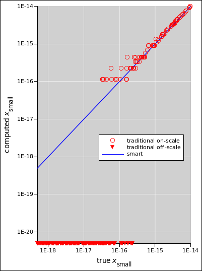
Figure 1 compares the smart formula (equation 2) with the not-so-smart formula (equation 18) over a range of conditions. The true xbig is between 1 and 8, such that log(xbig) is uniformly distributed. The true xsmall is between 10−14 and 10−19, such that log(xsmall) is uniformly distributed.
There is a range of many orders of magnitude where equation 2 produces the correct answers, but equation 18 produces wildly incorrect answers for xsmall. Cases where the incorrect answer is zero cannot be properly plotted on log-log axes, but are qualitatively indicated by downward-pointing triangles.
This is a super-simple example of a situation where you are given something that doesn’t at first glance “look like” a quadratic expression, but can easily be turned into one.
Let’s consider the equation
| (6) |
where z is small. This comes up in connection with the quadratic formula, and also in special relativity, as discussed in reference 1. Although equation 6 is just fine if you are doing algebra, it is grossly unsuitable if you want to evaluate it numerically. This is because of the infamous “small difference between large numbers” problem. You are much better off using equation 7 instead; it is algebraically exact and numerically well-behaved for all z≤1.
| (7) |
The reasoning behind equation 7 is the same as the reasoning behind equation 2, as discussed in section 1.
Let’s investigate another way of dealing with equation 6. You could expand the square root using a first-order Taylor series, namely:
| (8) |
whenever z is small compared to 1. This would give you a reasonably accurate answer if |z| is small enough. On the other hand, there is no real advantage to equation 8, because equation 7 is just as convenient and is less restricted.
If you want more accuracy than is provided by a first-order Taylor series, you should not assume that the best way forward is to use a higher-order Taylor series. Often there are other numerical methods that are better behaved. That is, they converge more quickly, giving higher accuracy with less work.
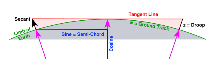
Here’s the scenario: A skilled surveyor sets up a horizontal line at his location. This is a very common surveying task. Often it’s a prerequisite for the tasks to follow. Horizontal means tangent to the equipotential curves of the earth’s gravitational field.
The surveyor has to account for the fact that the earth is not flat. It will droop away from the straight line in both directions. The question is, how much?
Here R denotes the radius of the earth and is represented in the diagram by the magenta arrows with arrowheads. Also w denotes the ground-track distance, measured by walking along the curved surface.
You can see that the droop z is:
| (9) |
That’s mathematically correct, but numerically ill-behaved when the droop is small compared to the size of the planet — which it usually is.
Equation 9 doesn’t look like a quadratic equation, but we can easily turn it into one. Using the trig identities you learned in high school, or re-examining the diatram and using the Pythagorean theorem you learned in elementary school, you can write:
| (10) |
where t = R tan(w/R).
Let’s expand equation 10 and put it in standard form:
| (11) |
The big root is therefore:
| (12) |
That’s not good for much other than finding the small root, which is what we care about:
| (13) |
This is mathematically exact, and is well behaved for large w, small w, and everything in between.
It is good practice to check the limiting cases. When w is small, t is well approximated by w, and equation 10 reduces to the familiar formula:
| (14) |
Similarly, when t is very large, equation 10 reduces to
| (15) |
which makes complete sense.
Significance: Equation 14 can be summarized as “7.84 cm per (km squared)”, or equivalently “8.00 inches per (mile squared)”.
Suppose you are constructing an airport runway, one mile long. One day the surveyor sets up at the south end and constructs a horizontal tangent line. He announces that you need 8 inches more dirt at the other end, to make it “straight”. At great expense, he hires heavy equipment to move the dirt around.
Then a week later he sets up at the north end and announces that the south end is now 18 inches too low. So again at great expense he moves the dirt around.
You need to fire that guy immediately, and hire somebody who knows how to account for the curvature of the earth.
You want the runway to be level. By definition that means that it follows one of the equipotential curves of the earth’s gravitational field. In particular: You don’t want it to be tangent to the potential; you want it to follow the curve of the potential.
Flat means planar. The runway cannot possibly be both planar and level. Note that the equipotential surface are also known as level surfaces.
Also: Horizontal means tangent to some equipotential surface. A flat plane that is tangent at one location won’t be tangent at other locations.
Let’s see what happens in a real-world equation. Here is an approximate equation that comes up in chemistry, when calculating the pH of an acid solution:
| (16) |
where
| (17) |
First, let’s see what happens if we try to solve that using the not-so-smart “textbook” version of the quadratic formula:
| (18) |
where in this case the variables are:
| (19) |
Let’s do a numerical example, in the case where the acid is strong but moderately dilute:
| (20) |
Let’s assume we arrived at the Ka value for our hypothetical acid by taking the average of various estimates. On this bases we estimate the uncertainty of Ka to be ±1×10⁴ or even more. The uncertainty in the concentration is negligible by comparison.
Plugging the Ka and CHA numbers into equation 18, we get
| (21) |
Now some people might decide on the basis of «common sense» that the number inside the square root could be rounded off to 3.210×10⁹. The uncertainty is so large that the sig-figs rules require us to round this number to a single digit, so carrying three extra digits «should» be plenty, or so the story goes. So let’s try rounding off and see what happens when we continue the calculation:
| (22) |
which is just completely wrong. Both of the alleged roots of the quadratic are negative. It is physically impossible for the [H+] concentration to be negative.
Analysis: It turns out that the «common sense» roundoff leading to equation 22 was a disaster. In this situation:
So now let’s switch to using the smart method. Equation 2 gives us:
| (23) |
where x2 is the desired answer. Rounding of intermediate results does not cause any problems. (This x2 value should not be taken as gospel, because equation 16 is only an approximation. It neglects the properties of the solvent. However, it’s in the right ballpark.)
It should have been obvious from the get-go that a 10−5 molar solution of a chemically-strong acid will have a pH of about 5.
We can write the kinetic energy as the difference between the total energy and the rest energy. This is valid in the high-speed limit, the low-speed limit, and everywhere in between.
| (24) |
Where ρ is the rapidity.
This is mathematically correct, but it is numerically ill-behaved at low speeds. It’s a classic “small difference between large numbers” disaster.
This is another example that doesn’t at first glance “look like” a quadratic expression, but can be turned into one.
This is discussed in detail in reference 1.
The ordinary sgn(x) function is defined to be −1 for all x<0, +1 for all x>0, and zero when x=0. The signum() function is same thing. Sometimes they are explicitly undefined when x=0.
None of the above are what we want for the quadratic formula. We need it to be either +1 or −1 when x=0. (Either one works.)
In most computer languages, you can implement the needed behavior as follows:
| (25) |
So all in all, the quadratic formula in computer-speak is:
|