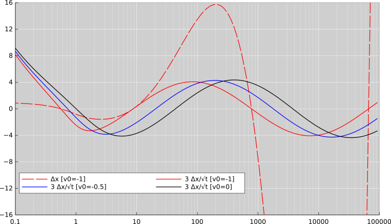
Figure 3: Oscillations in the Ratio Gun
We choose to study the following equation of motion:
| x•• = t / x (1) |
We will sometimes speak of the velocity and acceleration:
| (2) |
We classify the solutions as follows, depending on initial conditions:
Class C can be solved by inspection. It corresponds to the particular solution of the differential equation:
| x00 = | √ |
| t3/2 (3) |
A scaling argument tells us that all solutions will, at long times, converge ratio-wise to the particular solution. That is, for any solution x(t), we have
| (4) |
Let’s study how the solutions converge to the particular solution. To do that, we look at the residual, i.e. the position relative to the particular solution, namely:
| y := x − | √ |
| t3/2 (5) |
Numerical solutions indicate there is some interesting behavior to be found in the scaled residual, i.e. the residual demagnified by a factor of √t:
| (6) |
Solve for x:
| (7) |
First derivative:
| (8) |
Second derivative:
| (9) |
Substitute for the LHS using equation 1:
| (10) |
Eliminate x using equation 7:
| (11) |
The next step will be motivated by the expectation, based on the numerical integrations, that z may be periodic as a function of log(t) – not t itself. The second logarithmic derivative is:
| (12) |
So we rearrange equation 11 so as to bring the logarithmic derivative to the LHS:
| (13) |
We anticipate that if we expand the denominator in the last term on the RHS, expanding in a Taylor series to lowest order in z/t, the entire RHS will be equal to (−1/2)z to lowest order. Rather than using that approximate result at this time, we merely use it to motivate the following non-approximate re-arrangement, pulling the leading term to the front of the RHS:
| (14) |
For some purposes, it is useful to rewrite equation 14 as:
| (15) |
We observe that z≡0 at all times is a solution to this equation, corresponding to the particular solution.
All the calculations to this point are exact.
Equation 14 is a useful result. For all times greater than zero, it is formally equivalent to the original equation of motion, equation 1. It is somewhat more complicated-looking, but it is in some ways better behaved than equation 1, which has problems when x=0.
We observe that the RHS of equation 15 is well behaved, even if z and/or t goes to zero. The LHS is not particularly well behaved when t goes to zero, which tells us that ln(t) is in some sense a more “natural” variable than t itself, at early times in Class B and Class C. That is, we can integrate z′′ directly, where
| (16) |
where we define
| (17) |
More generally:
When z is large compared to t, as happens at early times in Class A, equation 16 can be approximated as
| (18) |
which can be solved by an exponential,
| (19) |
Numerical integrations show that in Class A at early times, z(t) is a straight line on log-log axes, with a slope of −1/2. The other possibility, +1/2, is not observed. This result is not particularly profound; the slope of −1/2 just corresponds to the factor of 1/√t in the definition of z.
Turning now to Class B, at short times we can use the following approximations
| (20) |
| (21) |
Again, this can be solved by an exponential, such that z(t) is a straight line on log-log axes, with a slope of ±1/2. In this case, only the positive-sloping solution is observed in the numerical integrations.
Also, again, this behavior is not particularly surprising, given the definition of z ... but it does at least serve as a check that our algebra is correct and our numerical methods are sound.
Everything below here is an approximation.
To further investigate the long-time behavior, we expand the RHS of equation 14 in a Taylor series, valid to first order in z/t.
| (22) |
In this expansion, the second term could be called the nonlinear term, since it is nonlinear in z. On the other hand, this same term should be considered the first-order term, since it is first order in the small quantity z/t. Perhaps this is clearer if we write the logarithmic derivative:
| (23) |
Based on the numerical integrations, as seen in figure 3, we expect z to be bounded at long times, so approximating things to second order (or even first order) in z/t should be a very good approximation when ln(t) is large. Dropping all but the first term on the RHS, we are left with the familiar equation for a harmonic oscillator:
| (24) |
That tells us we have sinusoidal oscillations when we plot z as a function of t on semi-log axes, or plot z as a function of τ on plain axes. The angular frequency and period in τ-space are:
| (25) |
Let’s compare this with the data. Note that in accordance with equation 25, this period in τ-space corresponds to a factor of exp(2π√2) i.e. approximately 7228 in t-space. Similarly, a half-period corresponds to a factor of exp(π√2) i.e. approximately 85.0197. Looking again at the nonlinearity in equation 22, we expect the half-period to be systematically longer when z/t is positive (because the magnitude of the curvature is less), and systematically shorter when z/t is negative.
Table 1 tabulates the zero-crossings of z, and the half-period of the oscillations, for the three different curves shown in figure 3.
| (for v0 = −1) | (for v0 = −0.5) | (for v0 = 0) | |||||||||||
| t @ z=0 | t ratio | : d | t @ z=0 | t ratio | : d | t @ z=0 | t ratio | : d | |||||
| —————————————- | —————————————- | —————————————- | |||||||||||
| 8.7402 | 20.493 | 43.4935 | |||||||||||
| } | 89.47 | } | 87.015 | } | 85.978 | ||||||||
| 781.995 | 1783.21 | 3739.48 | |||||||||||
| } | 84.9699 | : -585ppm | } | 84.997 | : -270ppm | } | 85.0085 | : -130ppm | |||||
| 66446 | 151567 | 317888 | |||||||||||
| } | 85.0203 | : +7ppm | } | 85.02 | : +3ppm | } | 85.0198 | : +1.5ppm | |||||
| 5.64926e6 | 1.28862e7 | 2.7027e7 | |||||||||||
In the table, the numbers under the heading d indicate where the half-period stands in relation to the expected asymptotic value, exp(π√2). This is not an indication of error or uncertainty, but rather shows the approach to the asymptote.
We see that at large t, the numerical results agree with the analytic results, within a small fraction of a percent. Indeed, locating the zeros of the oscillations is already a “small differences between large numbers” problem, demanding high accuracy from the numerical methods. The fact that the zeros themselves behave as expected, to good accuracy, is therefore an extremely sensitive check. The analysis serves as a check on the numerical methods and vice versa.
This system can be formalized in terms of a Lagrangian and a Hamiltonian that are time-dependent but otherwise more-or-less conventional. We start by assuming the following expression for the Lagrangian, and then show that it leads to the desired equation of motion. A potential-energy term logarithmic in x is plausible in light of the principle of virtual work, and is consistent with equation B.1.
| (26) |
It is always good to start with the Lagrangian, because we can then with confidence find the momentum that is canonically conjugate to x, namely
| (27) |
The Hamiltonian is then:
| (28) |
We then obtain the equation of motion via Hamilton’s equation:
| (29) |
Adopting the simplification m=1 we obtain equation 1, as desired.
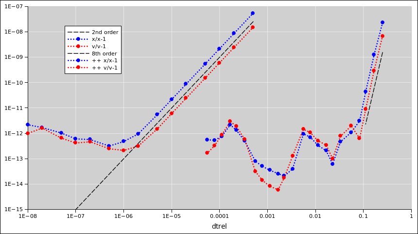
To test the accuracy of the numerical methods, we numerically integrated the equation for the particular solution (Class C), and then compared it to the closed-form solution. This is a demanding test, because of the infinite acceleration near t=0. We believe that if the integrator can handle this case, it can handle Class A and Class B with accuracy to spare.
The results are show in figure 4.
You can see that the higher-order method is many orders of magnitude faster, and a couple of orders of magnitude more accurate. However, the fastest behavior is not as accurate as one might have expected, and the most-accurate behavior is not as fast as one might have expected. Also, the approach to optimal accuracy is remarkably non-uniform.
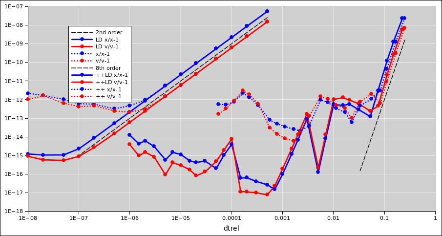
Things get even more interesting when we recompile the programs to use the long double data type for the critical computations. This data type is more-or-less universally available in contemporary hardware, and is supported by the C++ compiler since at least version 4.3. It allows numbers to be represented with more than three orders of magnitude more accuracy. Figure 5 shows these results (along with the plain-double results, for comparison).
You can see that the higher-order method does not benefit from the long doubles as much as might have been hoped. This is not surprising, since the code contains dozens and dozens of hard-coded “magic numbers” that were presumably computed with no more than double-precision accuracy.