*   Contents

• 1 Some Tips, Tricks, and Technicalities
  • 1.1 Beware Perverse Definitions
    • 1.1.1 Log(⋯)
    • 1.1.2 Floor(⋯) and Ceil(⋯)
    • 1.1.3 atan2(⋯)
    • 1.1.4 Int(⋯) and Rint(⋯)
    • 1.1.5 Summary of Rounding Functions
    • 1.1.6 Negative Exponentiation −A^B
  • 1.2 Date, Time, and Timezones
  • 1.3 Screwy Early Dates
  • 1.4 Beware Roundoff Error; Integers are Exact
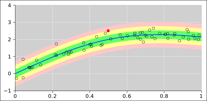
  • 1.5 Fuzzy Rounding
  • 1.6 Fenceposts, Lintels, Stairsteps, Treads, Risers, Chords, Derivatives, Integrals
    • 1.6.1 Duplicate Abscissas and Ordinates
    • 1.6.2 Discussion
    • 1.6.3 Deprecated: Subscripts and Superscripts
  • 1.7 Vector Cross Product
  • 1.8 Array Constants and Array Expressions
  • 1.9 A Bug + Workaround
  • 1.10 Reversing Rows and/or Columns
    • 1.10.1 Reversing Columns
    • 1.10.2 Reversing Rows
    • 1.10.3 Reversing Both Rows and Columns
    • 1.10.4 Discussion
  • 1.11 Curve Fitting; Linear Regression
  • 1.12 Convolutions
  • 1.13 Duplicating Treads and Risers
  • 1.14 Finding the Name of a Column
  • 1.15 Argmin and Argmax
  • 1.16 Computing a Reference to the Cell(s) of Interest
  • 1.17 Sorting Numbers
  • 1.18 Sorting Multi-Column Records
  • 1.19 Things We Know about Percentrank
  • 1.20 Counting Valid Numeric Elements
  • 1.21 Looking Stuff Up in a Table: vlookup and hlookup
    • 1.21.1 You Might Not Need a Lookup At All
    • 1.21.2 Avoid Multi-Column Lookups
  • 1.22 SQL Database Query : SELECT a Subset of the Data
  • 1.23 Plotting Multi-Dimensional Regions
  • 1.24 Plotting a Field of Vectors and/or Polygon
  • 1.25 Probability
    • 1.25.1 Triangular
    • 1.25.2 Rectangular
  • 1.26 Plotting Stairsteps, e.g. Cumulative Probability
  • 1.27 Plot Order aka Stacking; Plot per Series
  • 1.28 Plotting Arrowheads etc. in Screen Space
  • 1.29 Showing the Formulas aka Expressions
  • 1.30 Automatic Recalculation, Or Not
  • 1.31 Munging the Spreadsheet Document
• 2 Example: Combining Several Techniques: Probability Distributions
  • 2.1 Discrete Distribution: Two Dice
  • 2.2 Continuous Distribution: Gaussian
  • 2.3 Binomial Coefficients
  • 2.4 Binomial Distribution
• 3 References

1 Some Tips, Tricks, and Technicalities

1.1 Beware Perverse Definitions

1.1.1 Log(⋯)

Note the contrast:

This is a huge trap for the unwary. Constructive suggestion:

1.1.2 Floor(⋯) and Ceil(⋯)

Note the contrast:

This is another huge trap for the unwary. The only non-misleading workaround I know of is to avoid floor(x) and instead use -ceil(-(x)). See also section ‍1.1.4.

Meanwhile, the exist two spreadsheet functions, ceil(⋯) ceiling(⋯), which is a recipe for endless confusion. Spreadsheet ceil(⋯) is consistent with POSIX ceil(⋯); both round toward positive infinity. In contrast, ceiling(⋯) rounds away from zero.

1.1.3 atan2(⋯)

In c++, perl, maxima, and many other languages, atan2(sin(-3), cos(-3)) is equal to -3. However, alas, in a spreasheet, it is not. The order of the arguments is reversed. You have to write atan2(cos(-3), sin(-3)).

This will drive you crazy if you are trying to explain something to somebody, and you don’t know what language they will be using.

There is no workaround that I know of. You just have to write different code in different situations.

1.1.4 Int(⋯) and Rint(⋯)

• C++ rounds toward zero if you:
  • evaluate an integer expression such as (3/2).
  • assign a floating-point value to an int.
  • explicitly invoke the int(⋯) function.

  Apparently it always rounds toward zero AFAICT, no matter what the prevailing FPU rounding mode might be. Alas I don’t know if/where this is documented.

  As a consequence, when we evaluate y = int(x), the inverse image of y=0 is the entire open interval between −1.0 and 1.0, which is twice as big as the inverse image of any other integer.

  To avoid this inconsistency, when converting something to an integer, consider round(x). That is almost the same as ceil(x - 0.5).

  There is also a rint(⋯) function that rounds toward zero, plus infinity, minus infinity, or the nearest integer, depending on the prevailing FPU rounding mode.

• The spreadsheet int(x) function always rounds toward minus infinity. That means it is like POSIX floor(x). However, since the name is misleading, it is better to use −ceil(−x).

See also section ‍1.1.2

1.1.5 Summary of Rounding Functions

The situation is summarized in the following table:

The # symbol indicates that the spreadsheet function implements fuzzy rounding, as discussed in section ‍1.5. The ☠ symbol indicates that the name is deceptive because it conflicts with the C++ function name. When designing spreadsheets, I avoid the deceptive int(⋯), floor(⋯) and ceiling(⋯) functions. Instead I use the more portable substitutes indicated in the table.

1.1.6 Negative Exponentiation −A^B

Apparently the spreadsheet gives negation (i.e. unary minus) higher precedence than exponentiation, so -5^2 is equal to +25. Yuck. (Other computer languages, along with every math book on earth, give higher precedence to exponentiation.)

1.2 Date, Time, and Timezones

Time-of-day is stored as a number, measured in days; for example, 6:00 AM is stored as 0.25. Dates are just long times, measured in days since 30-Dec-1899, or equivalently 367 + days since 1-Jan-1901. Some examples and a couple of screwy exceptions are discussed in section ‍1.3.

With a few important exceptions, the date-related arithmetic and plotting is agnostic as to timezones. You can read in a bunch of dates in the form 3-Nov-2016 12:00 and plot them without caring what timezone they belong to. You can by fiat declare all the dates in your document to be UTC ... or you can equally well declare them to be in your local timezone ... or almost anything else, so long as you are consistent about it.

The exceptions are:

• The now() function always uses your computer’s local timezone.
• The date2unix(now()) function always uses UTC, measured in seconds since 1970, ignoring leap seconds. So the present time in UTC (measured in days, spreadsheet-style) is

          ="1-jan-1970"+date2unix(now())/86400
  

• On input, a date of the following form is accepted. It is a subset of an ISO standard form:

          2023-07-05T13:35:15Z
  

  The Z at the end denotes Zulu time (i.e. UTC). In this context, no other timezones are accepted, and the Z must not be omitted. The resulting cell value will be a date relative to UTC. It will not be converted to your local timezone, so it will not be consistent with the now() function. If you want consistency, you will have to write code to convert one or the other, using the offset described below.

  If you get a date with an explicit nontrivial timezone offset, you can convert to UTC by using string functions to split off the offset, then recombining things. For example, let cells A5:A7 contain:

          2023-07-05T16:39:39-07:00
          =iferror(search("-",A6,search(":",A6)),search("+",A6,search(":",A6)))
          =(mid(A6,1,A7-1)&"Z")-mid(A6,A7,99)
  

The offset of your local timezone relative to UTC (in days) is:

        =mod(0.5+now()-date2unix(now())/86400,1)-0.5

If that’s in cell A1, you can pretty-print it as:

        =if(A1<0,"−","+")&text(abs(A1),"h:mm")

1.3 Screwy Early Dates

Beware that all dates before 1-Mar-1900 are measured in days since 31-Dec-1899. That’s because some nitwit thought 1900 was a leap year. Dates after that are measured in days since 30-Dec-1899. Here are some key early dates:

1.4 Beware Roundoff Error; Integers are Exact

Suppose we want to count from 0 to 15 in steps of 1/3rd. The recommended approach is to use integers to count from 0 to 45 (in column A below) and then divide by 3. This gives the best possible result, because integers can be represented exactly. There will be some roundoff error, but there will be no accumulation of roundoff error. In particular, the rows in column B that should contain integer values will indeed contain exact integer values, as you can see by looking at every third row in the table.

In contrast, it is a bad idea for each row to iteratively add 1/3rd to the previous row, as in column D. We see that many of the numbers that are supposed to be integers are not. The 0 row is exact, of course. The 1 row is also exact; evidently the roundoff errors have cancelled out. However, the 2 row is off by a bit, although it’s not off by much; only −1 units in the last place (ulp).

In the 6 row, column D is off by −2 ulp, and by the time we get to the 8 row, it’s off by −4 ulp. Note that because this is floating point, the size of a ulp depends on the magnitude of the associated number.

Note that iterative addition is a very simple calculation. There are lots of more complicated calculations where the accumulated roundoff error is very much greater than 1 ulp.

The concepts in this subsection don’t have much to do with spreadsheets per se; mostly they apply to floating-point calculations in general. There’s a lot more that could be said about this. There are fat books on the topic of numerical analysis.

In contrast, the next subsection covers some similar issues that are inherently peculiar to spreadsheets.

1.5 Fuzzy Rounding

The fuzz issue is not super-important, because the errors it introduces are small. Meanwhile, floating point operations necessarily involve rounding, which introduces errors (on top of any fuzz-related errors). In multi-step calculations, the accumulated errors are commonly much larger that 1 ulp; the table above gives a hint of this. Decent algorithms do not assume the errors are 1 ulp or less; they are designed to cope with much larger errors.

fin

Figure ‍1: Fuzzy Rounding

You can see in figure ‍1 that one of the floating-point codes that should have been rounded up was not.

You can sorta imagine where this scheme come from. Somebody wanted to keep users from being surprised when numbers that were “almost” integers behaved strangely. Note that all the near-integers in the table in section ‍1.4 would seem to be exact if displayed with 14 or fewer decimal places, so the roundoff errors would not be super-obvious.

However, this is a fool’s errand. You can see in the table that out of 16 near-integers, there is only one case where fuzzy rounding has any effect at all. In 11 of the cases it isn’t necessary (because the number is already exact, or because the error is in a direction where it does no harm), and in 4 of the cases it isn’t sufficient (because the accumulated roundoff error is greater than 1 ulp). Even in the one case where there is some effect, it’s not clear that it’s a good effect. It creates a situation where ceil(x) is less than x, which seems like a Bad Thing.

All in all, the fuzzy rounding scheme adds to the complexity without solving any problems worth solving.

The only non-foolish procedure is to design your algorithms so that they are not sensitive to what’s going on in the 16th decimal place. If you need mathematical exactitude, use integers and rational numbers. The spreadsheet app uses the double data type for everything, which can represent integers exactly (if they’re not too huge). It can also express rational numbers of the form A/2^B, where A and B are integers. For example, 3/16ths is represented exactly.

Workarounds:

• If you don’t like the fuzzy spreadsheet function ceil(A1), function, you can use this instead:

          =(ceil(A1)+(ceil(A1)<A1))
  

• If you need to deal with near-integers, subtract a suitable fuzz-factor of your own choosing, then call ceil(⋯). For complex calculations, the fuzz-factor will be much greater than 1 ulp.
• If you need to deal with near-equality, compute the absolute value of the difference, and then compare that to a suitable fuzz-factor.

1.6 Fenceposts, Lintels, Stairsteps, Treads, Risers, Chords, Derivatives, Integrals

The term “fencepost problem” alludes to the proverbial long straight fence where there are N lintels held up by N+1 posts.

Figure ‍2: 4 Posts and 3 Lintels

This is relevant in many different computing situations, especially when an interval is divided into N subintervals (not necessarily all the same size) demarcated by N+1 endpoints. In particular, this is relevant to running sums, simple numerical integrals, simple numerical derivatives, and anything else where you might have stairsteps, treads, risers, or a threatened mismatch between posts and lintels.

1.6.1 Duplicate Abscissas and Ordinates

By far the slickest way to proceed is to put both the start and the end of each interval on the same row. So the row contains a lintel. The fenceposts are duplicated, because the right end of this row appears again as the left end of the next row.

        xleft   xright  yleft   yright  deriv   deriv
        1       2       f(1)    f(2)    d12     d12
        2       3       f(2)    f(3)    d23     d23
        3       4       f(3)    f(4)    d34     d34

This gives us a chordwise representation of the function f(). That is, it draws the chord line from (1, f(1)) to (2, f(2)).

You can calculate the numerical derivative as (yright-yleft)/(xright-xleft). It is a property of the interval, i.e. of the lintel, not a property of either fencepost. So put the value of the derivative in two successive columns.

This gives us a treadwise representation of the derivative f’(). That is, each row represents a tread, as the x variable advances. Risers happen between rows, as the f’() ordinate advances from d12 to d23.

You can devertialize the risers by shifting the top half a tread-width in one direction and shifting the bottom by half a tread-width in the other direction. If the derivative has a sharp corner in it (large second derivative) this doesn’t solve all the world’s problems, but it’s still a reasonable thing to do.

Often you want to do interpolation. That requires the abscissas to be strictly sorted. To arrange that, create two more columns, namely xleft*(1+delta) and xright*(1-delta), where delta is approximately the square root of the machine epsilon; that is, delta is about 1e-8. Then you can interpolate, using an N×2 array of abscissas and an N×2 array of ordinates.

Similarly the integrand is a property of the interval. The integral is the sum over intervals, summing the measure associated with the intervals. This allows you to find the resulting integral at the endpoints of the interval.

1.6.2 Discussion

• Everything discusses above applies to arrangements that are effectively one-dimensional. In two or more dimensions, e.g. dividing a sphere into octants, things get much more complicated.
• In the calendar, there is no year zero. The year 1 AD immediately follows the year 1 BC, even though this is inconsistent with modern notions of how to construct a number line.
• The ancient Romans counted intervals from start to end inclusive, which seems weird.
• Here’s another example of weird inclusive counting: In music, there are only 7 notes per diatonic octave, even though the name octave means 8. The eighth note is logically the beginning of the next octave. In particular, two octaves is not a 16th interval but rather a 15th. Three octaves is a 22nd. The formula is 3N+1. It’s off by one relative to modern notions of how to count.
• Beware that counting is different for a fence that forms a closed loop. Then you have N lintels supported by only N posts. For example, a circle can be divided into four quadrants, demarcated by four points.

1.6.3 Deprecated: Subscripts and Superscripts

The following is not very convenient. Use the methods outlined in section ‍1.6.1 instead.

• Number the posts from 0 to N inclusive, for a total of N+1 posts.
• Number the lintels from 0 to N−1 inclusive, for a total of N lintels. This is conventional in most modern computer languages.

  As a corollary, this means that each lintel is indexed accoreding to the post at the left end of the lintel, i.e. the lesser-numbered of the two posts that hold that lintel.

Format all the lintel-values as subscripts, and all the post-values as superscripts. This makes it easier to visualize the idea that the lintels fall between the posts. Alas the contrast between subscripts and superscripts is not as striking as one might have hoped, but it’s better than nothing. The goal is to get a spreadsheet that looks something like this:

1.7 Vector Cross Product

Let’s assume you have column vectors, not row vectors. Put the formula in the top cell of the result. Replace V$1 by the top of one of your vectors (two places), and W$1 by the top of the other (two places). Be sure to spell it with a $ sign in front of the row-number. Then fill down into the remaining cells of the result.

  =offset(V$1,mod(1+row($A1)-row($A$1),3),0)*offset(W$1,mod(2+row($A1)-row($A$1),3),0)
  -offset(V$1,mod(2+row($A1)-row($A$1),3),0)*offset(W$1,mod(1+row($A1)-row($A$1),3),0)

Even though the formula mentions cell A1, we do not care what (if anything) is there.

1.8 Array Constants and Array Expressions

In typical spreadsheets, curly braces are used to denote an array constant, for example {1,2,3} is a horizontal array. Similarly, {5;6;7} is a vertical array constant. Continuing down this road, {11,12,13;21,22,23;31,32,33} is a 3×3 matrix constant. The general rule is that commas are used to separate values on any given row, while semicolons are used to separate rows.

Here are some example of how this can be used:

• Cells: You can enter an array constant or array formula into an array of cells. As an example of entering an array constant, highlight cells A1:C1, then type ={1,2,3} and hit <ctrl-shift-enter>. As an example of an array formula, highlight cells A2:C2 an then type transpose(D1:D3) and hit <ctrl-shift-enter>.
• Linest: Consider using array constants when you are using a spreadsheet for least-squares fitting aka linear regression. Array constants can be used in connection with the linest(...) function. This provides a concise way of defining families of functions, such as the polynomial basis, the Fourier basis, et cetera. This sometime results in a dramatic reduction in the number of columns in the spreadsheet. An instance of this can be found on the polynomial-fancy page of reference ‍1; for a discussion of this example see reference ‍2.
• Range of numbers: There exists an idiomatic way of generating an array of consecutive integers in an array formula. As an example, here is a formula to calculate the sum of the first ten integers:

                  =sum(row($A$1:$A$10))
                  (not necessarily entered as an array formula)
  
  To generate <nval> values starting from <start>:
                  =row(offset($A:$A,start-1,0,nval,1))
  

  Additional applications of this idiom can be found below.

• Hamming weight, Hamming distance, and parity: You might think these functions would be built in, but they are not, so far as I can tell. I wrote functions to do this. They make good use of the aforementioned range-of-numbers idiom.

      Hamming weight      =sum(bitand(1,C9/2^(row($A$1:$A$64)-1)))
      Hamming distance    =sum(bitand(1,bitxor(C9,C10)/2^(row($A$1:$A$64)-1)))
      parity              =bitand(1,sum(bitand(1,C9/2^(row($A$1:$A$64)-1))))
  

• String match, aka string initial match: Count the number of character-positions in which the beginning of string C6 matches the beginning of string C7.

    String initial match  =sum(if(left(C6,row(offset($A:$A,0,0,len(C6),1)))=left(C7,row(offset($A:$A,0,0,len(C6),1))),1,0))
  

• Integrals including simple convolutions: Suppose we have a collection of 900 x-values, obtained perhaps by random sampling. We we want to treat those as delta functions. We convolve them with a Gaussian, to obtain a curve that is the sum of 900 Gaussians. We do not want our spreadsheet to have 900 rows and 900 columns. Indeed, it does not need to have 900 rows or 900 columns; we can store all 900 x-values in a 30 by 30 region.

          =sum(normdist(K10,AA$11:BD$40,K$4,0)*K$2)
  

  Explanation: The normdist() function ordinarily returns a scalar. If however you pass an array expression (constant or otherwise) as one of its arguments, it returns an array. This is an ephemeral array, not visible on the spreadsheet anywhere. In this example, the sum() collapses the ephemeral array, producing a scalar that fits in a single cell. Remember to enter the expression using <ctrl-shift-enter>.

Hint: If you ever enter something as a scalar when you should have entered it as an array, don’t panic. The formula is still there, and can easily be promoted to array-formula status. Highlight the area that is to be filled by the array, hit the <F2> key to move the focus to the formula bar, and then hit <ctrl-shift-enter>.

1.9 A Bug + Workaround

As we have seen in the examples above, you can do arithmetic involving array constants, for instance by highlighting cells A1:C1, then typing in =10^{1,2,3} and hitting <ctrl-shift-enter>. This will put the values 10, 100, 1000 into the three cells.

Obviously you can compute the maximum of these three cells using the expression max(A1:C1), and store this result in a single cell such as A3.

Logic suggests that you can do the same thing on the fly, by entering the combined expression max(10^{1,2,3}) into a single cell such as B3.

However, beware: Due to a bug in current versions of the gnumeric spreadsheet program, and possibly other programs as well, if you try in the normal way, you will get a numerically-wrong answer. See reference ‍3.

As a workaround for this bug, you can get the right answer by entering the formula =max(10^{1,2,3}) as an array formula using <ctrl-shift-enter>. There is no good reason why <ctrl-shift-enter> should be needed in this situation, because we are entering an ordinary scalar-valued expression, equivalent to the expression in the previous paragraph (which did not require <ctrl-shift-enter>).

1.10 Reversing Rows and/or Columns

1.10.1 Reversing Columns

Suppose you have data in columns B through E, and you want to make a copy with the columns in reverse order. You can use the following:

        =offset($B2,0,column($E2)-column(B2))
                 |            |          |
                first        last       first
                column       column     column

I prefer offset, but you can use index() instead if you want. It starts counting at 1, whereas offset() starts counting at 0. Also, index requires an array as its first argument, while for present purposes offset requires a single cell as its first argument (since we want each call to offset to yield a single cell).

        =index($B2:$E2,1,1+column($E2)-column(B2))

Fill across to cover all the columns of interest. Fill down if there are multiple rows in each column. (This is not meant to be entered as an array formula.)

1.10.2 Reversing Rows

Similarly, to reverse rows:

        =offset(B$2,row(B$5)-row(B2),0)
                 |       |
                top    bottom
                row     row

or perhaps equivalently

        =index(B$2:B$5,1+row($B$5)-row($B2),1)

Fill down to cover all the rows of interest. Fill across if there are multiple columns of in each row. (This is not meant to be entered as an array formula.)

1.10.3 Reversing Both Rows and Columns

Finally, to flip both the rows and the columns all at once (i.e. a 180^∘ rotation):

        =offset($B$2,row(B$5)-row(B2),column($E2)-column(B2))
                  |       |                    |
                upper   upper                lower
                left    right                left

Fill down and fill across to cover all the rows and all the columns.

1.10.4 Discussion

It would be super-nice to be able to express the reverse as an array expression, but I have not found a way to do this. The index() and offest() functions do not appear to tolerate array expressions in their second or third arguments.

Reversing turns out to be important in connection with convolutions.

Multiplying two polynomials is convolution-like. Start by reversing one of the multiplicands (i.e. reversing the list of coefficients). Then use a formula like this:

        =sumproduct(offset(M4,0,0,1,1+AA$2),offset($AC3,0,0,1,1+AA$2))

Another important application arises in connection with a band plot such as in figure ‍3. Ideally it would be possible to make such a plot using the "fill to next series" feature of the spreadsheet program, but in older versions of gnumeric that has bugs. It is better to use the "fill to self" feature. This requires tracing the top of each band in the normal order, then tracing the bottom of each band in reverse order.

Figure ‍3: Band Plot

1.11 Curve Fitting; Linear Regression

See reference ‍2.

1.12 Convolutions

Here is an example of a convolution:

          npts:   8                       =sumproduct(offset($B$10,max(0,row(A1)-$C$7),0,min(row(A1),2*$C$7-row(A1))),offset($D$10,max(0,$C$7-row(A1)),0,min(row(A1),2*$C$7-row(A1))))
                          =offset($C$10,$C$7-row(A1),0)
  label
  0       0       0       0               0
  1       1       1       1               0
  2       1       1       1               1
  3       1       1       1               2
  4       1       1       1               3
  5       1       1       1               4
  6       1       1       1               5
  7       0       0       0               6
  8                                       5
  9                                       4
  10                                      3
  11                                      2
  12                                      1
  13                                      0
  14                                      0

where cell $c$7 contains the number of points in each vector (npts: 8) and the first vector begins at $b$10 and the second begins at $c$10. The reverse of the second vector begins at $d$10.

1.13 Duplicating Treads and Risers

Suppose you have a row of data: 1, 2, 3, et cetera. You would like to plot each data item twice. Usually the best way to do this is to put the duplicates in adjacent rows as discussed in section ‍1.26.

However, sometimes you might want to keep everything in a single row, and just have twice as many cells in the row, so that the row reads 1, 1, 2, 2, 3, 3, et cetera. This situation can easily arise if you want to draw a stair-step function. The vertical risers require you to duplicate the abscissas, and the horizontal treads require you to duplicate the ordinates.

The index function can do this for you:

        =index($I11:$W11,1,1+(column(I11)-column($I11))/2)

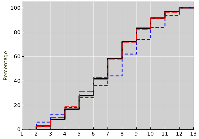
Note that stair-steps arise if you are plotting the cumulative probability for a discrete distribution, such as in figure ‍4.

Figure ‍4: Cumulative Probability for Two Dice

1.14 Finding the Name of a Column

The column(M7) function returns the address of the given column; in this example, “M” is column number 13. If however you want the column letter, aka the column name formatted as a letter, you have to work harder. Here’s the recommended expression:

        =substitute(address(1,column(M7),4),"1","")

Explanation: The row number (“7”) here is irrelevant. The column(M7) function returns 13, ignoring the row number. The address(...,4) function returns an address, namely the text string “M1”. The “4” here tells it to return a relative address (i.e. without any $ signs). Lastly, we get rid of the “1”.

Here’s one rationale for doing something like this: Suppose you want to format a message that refers to the column in which cell M7 was found. Next, suppose you cut-and-paste cell M7 to a new location such as N8. The result of the recommended expression will change accordingly; the new result will be “N”. In other words, the recommended expression is translation invariant – whereas a simple string constant (in this case “M“) would not be.

In some cases there are simpler ways of achieving translation invariance, as discussed in section ‍1.16.

1.15 Argmin and Argmax

Use the match(needle,haystack,0) to return a relative row number. A result of 1 corresponds to the first row in the haystack range. In particular, argmax is match(max(haystack),haystack,0) and argmin is match(min(haystack),haystack,0).

The result can then be used in the index(range,relRow,relCol) function to fetch a value. Equivalently, it can be used in the offset function, provided you subtract 1.

1.16 Computing a Reference to the Cell(s) of Interest

• Usually the simplest and best approach to use the match() function to create a reference to the cells you want.
• It is a dubious practice to cobble up cell addresses by concatenating non-constants such as the row-letter computed in section ‍1.14. This can be made to work correctly, but it’s usually messier than the previous suggestion.
• It is an even worse practice to cobble up cell addresses by concatenating string constants and then using the indirect() function. The problem is that the constants do not “track” properly if stuff gets relocated. That is to say, they are not translation invariant.

1.17 Sorting Numbers

To sort numbers in ascending order:

        =small($D$4:$D$99,1+row($D4)-row($D$4))           <E>

where <E> means you can enter it as a plain old scalar formula (not array formula).

1.18 Sorting Multi-Column Records

Step 1: To get an array of indices, apply the following to the sort key, to encode the key and the corresponding row number. In this example, the input data starts at D$4.

        =round(percentrank(D$4:D$99,D4,20)*(count(D$4:D$99)-1))+(row($d4)-row($d$4))/1000   <E>

Format that with three decimal places.

See section ‍1.19 for a discussion of the percentrank function. Let N denote the number of valid elements. Multiplying the prank by N−1 (and rounding) gives the rank as an integer (with N possible values from zero to N−1 inclusive). We use the integer rank as our sort key. The rest of the expression uses the fraction part to encode the index, to remember where this element was before sorting.

Step 2: Sort the indices. Suppose the keys are in column A and we want the sorted results in column B:

        =small(A$4:A$99,1+row($B4)-row($B$4))
or
        =large(A$4:A$99,1+row($B4)-row($B$4))

Then extract the row number, which serves as an index:

        =round(mod(B4,1)*1000)

Or combine the two previous steps, to calculate the index directly:

        =round(mod(small(A$4:A$99,1+row($B4)-row($B$4)),1)*1000)
        =round(mod(large(A$4:A$99,1+row($B4)-row($B$4)),1)*1000)

Then you can use offset(...) to fetch all the sorted field(s) you want, not just the sort key field.

        =offset(x!D$2,$B2,0)    <E>

Fill that across (to pick up all fields) and down (to pick up all records) as required.

1.19 Things We Know about Percentrank

• Calling percentrank(haystack, needle, precision) returns a result (called the prank) in the interval [0,1] (not [0,100]).
• If there is a tie, the prank is the lowest rank that could be assigned to any member of the tied group.

  You can check for ties by looking at the ascending and descending pranks; they should add up to unity:

          =percentrank(D$2:D$6,H2,20)
          =percentrank(iferror(-D$2:D$6,"x"),-H2,20)
  

• Let N denote the number of valid elements in the haystack. Blank cells and string-valued cells are ignored, and don’t contribute to the value of N. See section ‍1.20 for a way of evaluating N.
• Suppose some element with value V is part of an M-way tie, and suppose it corresponds to some prank we denote R_low. Then if the needle is infinitesimally larger than V, its prank is R_high = R_low + (M−1)/(N−1).

  This makes sense insofar as it is 1/(N−1) less than the prank of the next-larger element of the haystack, i.e. R_next = R_low + M/(N−1)

• If the needle falls between two elements of the haystack, the prank is computed by linear interpolation, starting from R_high and ending at R_next, so as the needle varies over the interior of the open interval, the prank changes by 1/(N−1). (The change is not 1/N, which would be a fencepost error.)
• Therefore if there are no ties, the prank is a continuous function of the needle-value. A stronger statement is: If and only if there are no ties, not counting a possible tie for top rank, the prank is a continuous function of the needle-value.
• The smallest element of the haystack has prank 0.
• If the largest element is not tied, it has prank 1.
• If the median element is not tied, it has prank 0.5.

1.20 Counting Valid Numeric Elements

To find the number of valid numeric elements in a region, ignoring strings, empty cells and #ERROR cells, use the following, entered as an array formula:

        =count(B15:C17)
or equivalently
        =sum(iferror(B15:C17-B15:C17+1,0))      (array formula)

If you want something that does not ignore #ERROR cells, try something like this:

        =rank(max(B15:C17),B15:C17,1)+sum(if(B15:C17=max(B15:C17),1,0))-1

If there are one or more errors anywhere in the range, the result will be an error. The type of the result error will match one of the input errors.

1.21 Looking Stuff Up in a Table: vlookup and hlookup

1.21.1 You Might Not Need a Lookup At All

• Instead of using vlookup() or hlookup() in “approximate” mode, often the interpolation() function is easier and better. Sometimes this is even true in “non-approximate” mode.

  Interpolation is very much more forgiving (compared to lookups) if the abscissas aren’t exact.

  Beware that the interpolation() function insists on performing extrapolation if it runs out of ordinates. Blank ordinates are not the same as zeros, but you can fix this by writing “0+range” instead of simply “range” in the second argument, as in the example in section ‍1.21.2.

• If your abscissas are evenly spaced, a simple offset() is simpler and incomparably more efficient.

1.21.2 Avoid Multi-Column Lookups

Avoid using a multi-column area as the second argument of vlookup(), or more to the point, avoid using any number other than 1 as the third argument (the readout column). That’s because anything that requires you to count columns is bug-bait. In particular, if somebody ever wants to insert or remove a column from your table, it will break things.

Instead, use a one-column area as the second argument, set the third argument to 1, and also set the fourth argument to 1 so that vlookup() returns an index. Then feed that index to offset() to grab the desired element from the appropriate column. This makes your spreadsheet vastly more reliable, more debuggable, more maintainable, and more extensible.

For example, instead of:

        =vlookup(B19-$H$12,$B$19:$I$138,8,1)

you might be a lot happier with:

        =offset($I$19,vlookup(B19-$H$12,$B$19:$B$138,1,1),0)

and even happier with:

        =interpolation($B$19:$B$138,0+$I$19:$I$138,B19+$H$12)

Similary words apply to hlookup().

1.22 SQL Database Query : SELECT a Subset of the Data

Sometimes you want to select a subset of the original data, and put it into a new region without gaps. This is called a query. You might want to run multiple queries against the same original data.

As a particularly simple example, suppose you want to select all the valid data, squeezing out non-numerical entries (such as blank cells, strings, and #ERROR cells) to produce a result with no gaps.

Suppose the original data is in cells a6:c37. That’s a total of N=32 rows. Columns B and C can be used for some related (or unrelated) purpose.

Let’s skip a column (D) for clarity.

Use column E to keep a running sum of how many times the selection criterion is met. There has to be a zero in cell E5. Then in E6 we use the formula:

        =if(count(A6), round(E5)+1, E5+1e-9)

where the first argument to the if(,,) statement is the criterion; it should evaluate to true whenever the criterion is met, and false otherwise. Note the 1e-9 which is necessary to make sure the elements in this column are strictly sorted, as required by vlookup(). The idea is that each valid entry gets an integer sequence number, while invalid entries get a non-integer.

This is not an array formula. Fill down so there are N−1 rows of this formula (following the zero in cell E5).

Then in the next column (F), find where each successive match occurs. Vlookup returns a 0-based index into the original data. When exact matching is in effect, it returns -1 when there is no match.

        =vlookup(1+row()-row($F$6),E$6:E$24,1,0,1)

The second argument to vlookup is the column to be searched. The fifth (i.e. last) argument says we want an index, which means the third argument is irrelevant, but it is not ignored, so it has to be 1. The fourth argument is 0 which means we don’t want an approximate match; instead we insist on an exact match. (Otherwise it would be much harder to deal with the end of the result region, where there are no valid matches.)

Then in the next column (G) we collect the results.

        =if($F6>=0,offset(B$6,$F6,0),"xxx")

That can be filled down and across as much as you like. Filling across picks up data from columns B and C, but the validity decision is still based on column A.

1.23 Plotting Multi-Dimensional Regions

When plotting, in the simplest case, the ordinate of the plot is a one-dimensional spreadsheet region, by which I mean a region that is either N rows by 1 column, or 1 row by N columns. (Ditto for the abscissa, if any.)

However, it is perfectly possible for the ordinate (and/or abscissa) to be a rectangular region, with M rows and N columns. The region is read in row-major order; that is, every cell in a given row is read out before advancing to the next row. For example, the region A1:C10 contains 30 elements, in the following order A1, B1, C1, A2, ⋯ B10, C10.

1.24 Plotting a Field of Vectors and/or Polygon

It is reasonably straightforward to plot a set of arbitrary line segments (disconnected from each other). Similarly it is reasonably straightforward to plot a set of arbitrary triangles or other polygons.

The basic idea is to plot them as an ordinary “XY lines” plot. To separate one item from the next, put a non-numeric value in the list of abscissas and/or ordinates. A blank will do, it is more readable if you use a string such as “break” or “X”.

This idea combines nicely with the rectangular regions discussed in section ‍1.23. To plot N line segments, use three columns of N rows for the abscissas (tail.x, tip.x, and “break”) plus three columns for the ordinates (tail.y, tip.y, and “break”).

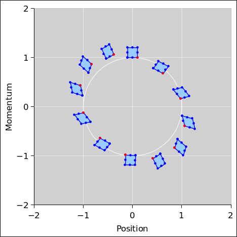
Similarly, to plot N quadrilaterals, use six columns of N rows; the first four define the corners, the fifth returns to the starting point to close the last side, and the sixth is the “break”. An example is shown in figure ‍5.

Figure ‍5: Quadrilaterals : Phase Space of a Harmonic Oscillator

If you don’t need to close the last side, you can get by with only five columns. For an example, see figure ‍9 in section ‍2.1.

1.25 Probability

1.25.1 Triangular

For a triangular distribution with a mean of 0, a height of 0.5, and a HWHM of 1 (HWBL of 2), the probability density distribution is:

        =(0.5-abs(C5/4))*(abs(C5)<2)

This assumes you have already, in a previous step, normalized the data by subtracting off the mean and dividing by the HWHM. Furthermore, you will have to postmultiply the density by the inverse of the actual HWHM, so that the area under the curve will be unity.

The corresponding cumulative probability distribution is:

        =if(abs(C5)<2,0.5+C5/2-C5*abs(C5)/8,(sign(C5)+1)/2)

1.25.2 Rectangular

For a rectangular distribution with a mean of 0, a height of 0.5, and a HWHM of 1 (HWBL also 1), the probability density distribution is:

        =(abs(C5)<1)/2

This assumes you have already, in a previous step, normalized the data by subtracting off the mean and dividing by the HWHM. Furthermore, you will have to postmultiply the density by the inverse of the actual HWHM, so that the area under the curve will be unity.

The corresponding cumulative probability distribution is:

        =if(abs(C5)<1,0.5+C5/2,(sign(C5)+1)/2)

1.26 Plotting Stairsteps, e.g. Cumulative Probability

For a discrete distribution, such as we get from rolling a die, cumulative probability is a stairstep function. Suppose there are N steps. Depending on details of the desired appearance, this will correspond to either N treads and N+1 risers, or perhaps N+1 treads and N risers. Either way, there is a nice representation using N+1 rows of four columns: two columns for the abscissas, and another two columns for the ordinates. Each row represents one tread: It has two unequal abscissas (the left edge and the right edge of the tread) and two equal ordinates (since the tread is horizontal).

For an example, see section ‍2.1.

1.27 Plot Order aka Stacking; Plot per Series

In order to understand what gets plotted in front of what, it helps to know some terminology. However, the terminology for graphical objects is maddening. You might imagine that words like graph, chart, and plot should mean pretty much the same thing ... but in this context they don’t. I write these words in small caps to indicate that they are codewords.

Gnumeric doesn’t even use its own terminology consistently. The popup for customizing a graph and its contents is entitled «Customize Chart» whether or not the graph contains zero, one, or many charts.

Here is a subset of what is going on, even when you try to do something simple. Suppose we are making an XY plot of some data:

1.  ‍ ‍ ‍The top-level object is called a graph.
   1.  ‍ ‍ ‍The graph can have zero or more graph-titles.
   2.  ‍ ‍ ‍The graph can have zero or more charts.
      1.  ‍ ‍ ‍Each chart can have zero or one backplane.
      2.  ‍ ‍ ‍Each chart can have zero or more legends.
      3.  ‍ ‍ ‍Each chart can have zero or more chart-titles.
      4.  ‍ ‍ ‍Each chart that contains an XY plot can have one or more X-axes. The first X-axis cannot be deleted, and controls the X-scale factor for all plots (and their series) on this chart. Additional X-axes, if any, are basically just ornamental.
         1.  ‍ ‍ ‍Each X-axis can have zero or one major grid.
         2.  ‍ ‍ ‍Each X-axis can have zero or one minor grid.
         3.  ‍ ‍ ‍Each X-axis can have zero or one axis-label.
      5.  ‍ ‍ ‍Ditto for the Y-axes.
      6.  ‍ ‍ ‍Each chart can have zero or more plots of axis-compatible type. Axis-compatibility means you can add an XY plot on top of an XY plot, but you cannot add a Radar plot on top of an XY plot or vice versa. Remember that one set of axes controls every plot within the chart. You might imagine that the type of the chart would be a property of the chart itself, but no, it is controlled by the type of the first plot within the chart.

         In contrast, the size and position of the plots is controlled by properties of the parent chart – not by the axes, and not by the plots themselves. Don’t ask me to explain this.

         1.  ‍ ‍ ‍Each plot can have zero or more series.  ‍ ‍ ‍ ‍
             ‍ ‍ ‍ ‍
            

            ∗ ‍ ‍ ‍ Each series can display data using lines.

            ∗ ‍ ‍ ‍ Each series can display data using pointlike symbols.

            ∗ ‍ ‍ ‍ Each series can display data using shaded regions.

Now, you might imagine that the drawing routines would recurse through the objects pretty much as shown above. In particular, you might imagine that gnumeric would finish drawing one series before going on to the next. However, that’s not how it actually works. The innermost loops are done “inside out” as explained below. This is completely undocumented, indeed contrary to the documentation.

The actual behavior can be outlined in pseudocode, as follows:

     foreach plot in chart.children {
        foreach drawable in [line, symbol] {
           foreach series in plot.children {
              draw(series, drawable)
           }
        }
     }

In English, that means that within each plot, the lines (for all the series) are drawn in order, and then the symbols (for all the series) are drawn in order. All of the lines wind up behind all of the symbols. The stacking of the lines (relative to other lines) is controlled by the order of the series as they appear in the user interface, and similarly for the stacking of the symbols (relative to other symbols). However, within a plot, there is no way to draw a line on top of a symbol ... even if you have one series that uses only lines and another that uses only symbols. No amount of re-ordering the series within a plot will change this.

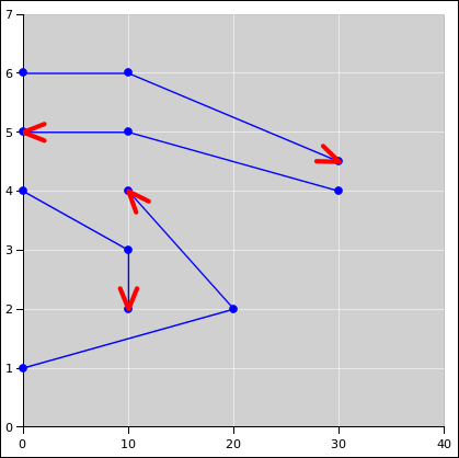
This ordering may not be what you want. (An example arises when plotting arrowheads on top of target symbols, as discussed in section ‍1.28.) In such a case, the only way to make progress is to use more than one plot, and order the plots appropriately. You can achieve quite fine control over the “stacking” – i.e. the order of plotting – by putting each series in its own plot. Use one series per plot, i.e. one plot per series.

For even finer control of the plot order, don’t rely on a single series to draw both lines and symbols. Instead, split it into two series looking at the same data. One series displays the lines, while the other series displays the symbols.

This business of creating more than one plot would be a lot more practical if it were possible to move a series from one plot to another, but evidently that is not possible. The buttons that move a series up and down in plot order get stuck at the boundary between plots.

While we’re on the subject: What would help most of all is the ability to copy-and-paste a series ... and also copy-and-paste an entire plot (along with all its series). This includes being able to copy a series from one plot and paste it into another. The ability to copy-and-paste (not just cut-and-paste) has innumerable applications. It is very common to want a new curve that is just like an old curve, with minor modifications.

1.28 Plotting Arrowheads etc. in Screen Space

It is important to distinguish between data space and screen space.

• Data space is abstract. In (say) a plot of force versus time, data space might have units of newtons in one direction and seconds in the other direction.
• Screen space is direct and concrete. It is the physical distance on the screen. It might have units of cm (or pixels) in both directions. Crucially, the units are the same in all directions.

There are some things such as arrowheads that clearly need to be plotted in screen space, not data space. You want the arrowhead shape to be preserved, even if it is rotated by some odd angle. The idea of rotation makes sense in screen space, but violates basic requirements of dimensional analysis in data space, where there is not (in general) any natural metric, i.e. not any natural notion of distance or angle.

In figure ‍6, the extent of the plot in the x direction is more than fivefold larger than the extent in the y direction. The arrowheads would be grossly distorted if we tried to draw them in data space without appropriate correction factors.

Figure ‍6: Drawing Arrowheads in Screen Space

Although typical spreadsheet apps do not provide easy access to screen space, we can work out the required transformations. The first step is to figure out the metric. We know the metric in screen space, and we use this to construct a conversion metric for data space. Let’s denote data space by (x, y) and screen space by (u, v).

It must be emphasized that the arc length ds is the same in both equation ‍3 and equation ‍4. It is the real physical arc length on the screen.

You can determine the coefficients a and b as follows: Lay out a rectangle on the chart. Let the edges of the rectangle be (Δu, Δv) in screen space, and (Δx, Δy) in data space. Then the needed coefficients are:

The conversion metric defines a notion of length and angle in data space. Given a line segment in data space, we can construct a tangent unit vector with the same orientation ... where “unit” refers to its length in screen space. We can also define a transverse unit vector, perpendicular to the line segment ... where “perpendicular” refers to its angle in screen space.

It is then straightforward to construct arrowheads and other objects in terms of the tangent unit vector and the transverse unit vector.

If you change the size of the chart or rescale the axes within a chart, you will have to recompute the a and b coefficients in accordance with equation ‍5. This is a pain in the neck if the axis bounds are being computed automatically.

Before you start plotting arrowheads, be sure to read section ‍1.27. You may want to use the one-plot-per-series construction for your vectors and arrowheads.

The spreadsheet code to do this is cited in reference ‍4. In this example, the plotting area is square, and the edge-length of the plotting area is taken as the unit of distance in screen space. The size of the arrowheads is 1/20th of this distance. This is of course only an example; any other distance could be used in accordance with equation ‍5.

1.29 Showing the Formulas aka Expressions

There are several ways to see the formula aka expression in a cell (as opposed to the value obtained by evaluating the expression).

1. The ctrl-‘ key toggles between ordinary show-value mode and show-formula mode. Hold the control key while hitting grave-accent key (which is typically just to the left of the “1” key).
2. The get.formula(X1) function will display the formula in cell X1, including the initial “=” sign. Note that if the cell contains a constant such as 123 (as opposed to a formula such as “=123”) the get.formula() displays nothing.

   I use this a lot. It is useful in pedagogical situations, where you want people to be able to see the formula and the value at the same time. It is also useful as a way to put formulas and/or addresses into a .csv file, which (as the name suggests) nominally only includes values. There are lots of good reasons why you might want formulas and/or addresses in .csv files.

3. The expression(X1) function is the same, except that it does not display the initial “=” sign.
4. Clicking on any given cell displays the cell’s formula in the formula bar.
5. Double-clicking on any given cell displays the cell’s formula in-place (as well as in the formula bar).

1.30 Automatic Recalculation, Or Not

Sometimes it is useful to turn of the “Automatic Recalculation” feature. Examples include

• Situations involving iterative solutions, where you might want to observe the process step by step. See e.g. reference ‍5.

You can manually cause a new calculation at any time by hitting the <F9> key.

• This is obviously useful when Automatic Calculation is turned off.
• It is sometimes useful even when Automatic Calculation is turned on, for instance when dealing with random numbers. Every time you hit <F9> you get a new set of random numbers.

1.31 Munging the Spreadsheet Document

The default format that gnumeric uses for storing spreadsheet documents is structured as XML. Often there is gzip compression on top of that, but uncompressing it is super-easy.

(I have no idea what format excel uses.)

It is fairly easy to figure out what the XML means, and then to munge it using a text editor, or using tools such as grep, awk, perl, et cetera.

For example, suppose you want to have a plot with 35 curves on it. Configuring all of those using the point-and-click interface is unpleasant the first time, and even more unpleasant if you want to make a small change and then propagate it to all the clones. Therefore I wrote a little perl program that take one curve (aka Series) as a template and then makes N clones.

2 Example: Combining Several Techniques: Probability Distributions

2.1 Discrete Distribution: Two Dice

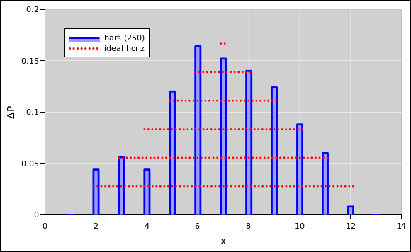
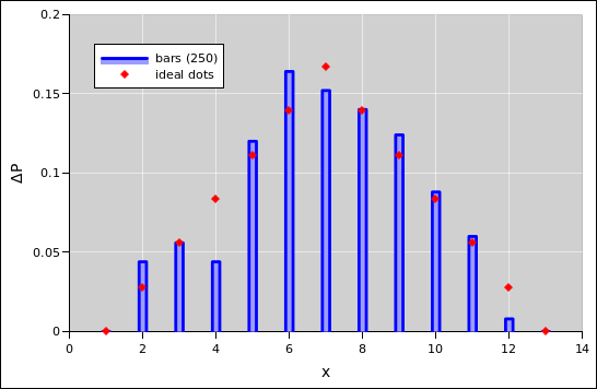
The spreadsheet in reference ‍6 calculates the probabilities for a pair of dice. Look at the “histo-2-efficient” worksheet.

Figure ‍7: Two Dice : Cumulative Probability		Figure ‍8: Two Dice : Probability Histogram + Triangle

Figure ‍9: Two Dice : Probability Histogram + Horizonal Lines		Figure ‍10: Two Dice : Probability Histogram + Dots

Note the following:

1. The offset() function is used to select a subset of the data. There are 1000 raw data points, and normally you would want to use them all, but just for fun in this special case only 250 are used to calculate the histograms.
2. The cumulative probability uses the stairstep technique discussed in section ‍1.26.
3. The histogram in figure ‍8 uses yet another trick: The nominal ordinate of the plot is zero. The histogram bar you see is the upper error bar. This technique seems cute at first glance, but it has a fatal flaw: The plot uses no markers and no line-code, so the trace does not show up in the legend in any reasonable way.

   Therefore it is better to use the approach seen in figure ‍9 and figure ‍10. They plotted the histogram as a bunch of quadrilaterals, using the techniques mentioned in section ‍1.24.

4. I am quite aware that the spreadsheet program has a built-in facility for producing histograms. It is OK in simple situations, but I continually find myself wanting to do something it can’t handle. The techniques in this example are just as easy to use, and much more flexible.
5. The cumulative probability distribution is calculated using an array formula, which is summed in place. This formula must be entered using control-shift-enter.

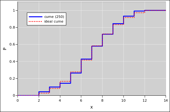
   For a continuous probability distribution, the right approach is to sort the data. Then the index (suitably normalized) is the cumulative probability, as a function of the data value. That is to say, there is a riser at every data point, and a tread between each two data points. See section ‍2.2 and reference ‍7.

   For discrete data, with relatively few categories, sorting is inefficient and unnecessarily complicated.

2.2 Continuous Distribution: Gaussian

Figure ‍11: Gaussian Cumulative Probability Distribution		Figure ‍12: Gaussian Probability Density Distribution

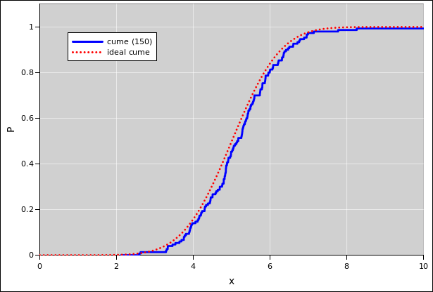
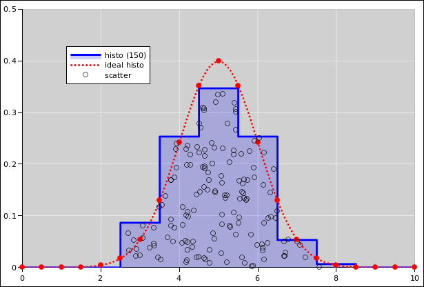
Figure ‍13: Gaussian Cumulative Probability Distribution		Figure ‍14: Gaussian Probability Density Distribution

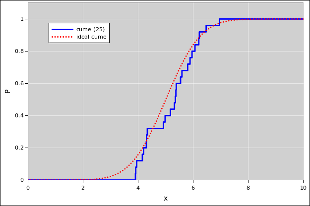
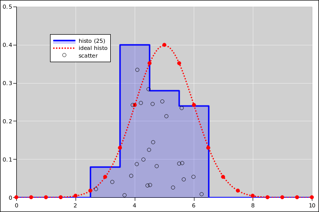
Figure ‍15: Gaussian Cumulative Probability Distribution		Figure ‍16: Gaussian Probability Density Distribution

See reference ‍7.

For plotting the cumulative probability distributions, the following statement comes in handy:

   =if(J8<1,small(offset($E$8,0,0,G$4),1+row($$E8)-row($E$8)),9e+99)

• Start with the raw data, a bunch of x-values, randomly drawn from some distribution.
• In a new column, sort them in order of increasing x, using the techniques set forth in section ‍1.17.
• The cumulative probability distribution is a stairstep function, in which event corresponds to a riser. For instance, the first event in the list corresponds to the riser going from count=0 to count=1. If there are N events, we normalize this so that the first riser goes from P=0 to P=1/N.
• Use an offset() statement so we can sort only a subset of the data if we wish.
• Use an if() statement so that we can achieve the proper asymptote P(x) = 1 for large x.
• There are no adjustable parameters. The empirical distribution of the data converges to the ideal distribution with no help from us.

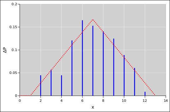
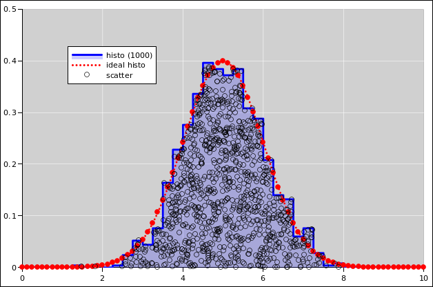
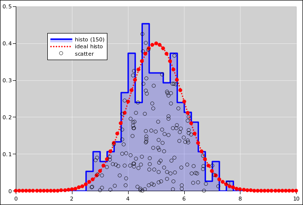
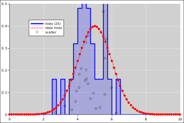
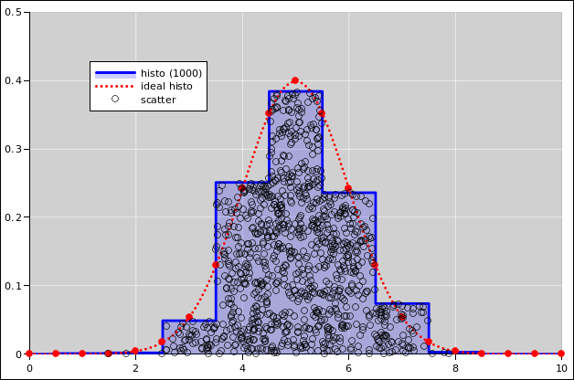
As for the probability-density histogram:

• There is an adjustable parameter here, namely the bin-width, i.e. the extent of the bin in the x-direction. If we have a huge number of points, the bin-width can be smaller.
• The histogram is a stairstep function, in which each bin corresponds to a tread.

  The support of each bin is a half-open interval of the form [L, R) such that the bin contains all events such that x is greater than or equal to L and strictly less than R. For continuous data, the chance that any data point falls exactly on a bin boundary is zero, but for discrete data this can become an issue, hence the careful definition of the bin-boundaries.

If the bin-width gets too small and there are not enough data points, the histogram becomes noisy. At some point a noisy histogram becomes hard to interpret; among other things, the idea of half-width at half-maximum becomes useless.

Figure ‍17: Gaussian Probability Density Distribution

Figure ‍18: Gaussian Probability Density Distribution

Figure ‍19: Gaussian Probability Density Distribution

2.3 Binomial Coefficients

The spreadsheet function combin(n, k) returns the binomial coefficient “n choose k”. For example:

For example:

2.4 Binomial Distribution

Here is a statement that produces a random integer according to a binomial distribution. In this example, there are 60 trials. (The number of trials is built into the statement.) The first argument to the binomdist function is the outcome. Here we use an array expression, using the range-of-numbers idiom mentioned in section ‍1.8. The second argument is the number of trials. The third argument is the probability of success per trial, which we assume is stored in cell $D$3. We use the sum function to count how many times the probability of a given outcome was less than the threshold, where the threshold is some random number stored in cell G7.

     =sum(if(binomdist(row($A$1:$A$61)-1,60,$D$3,1)<G7,1,0))

Suppose we use that formula 200 times, using a different random threshold each time. The results are shown in the following figures. See reference ‍8 for details.

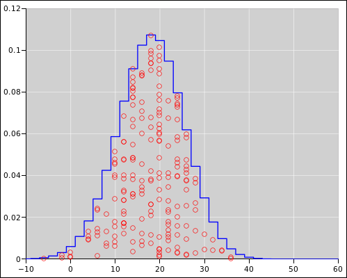
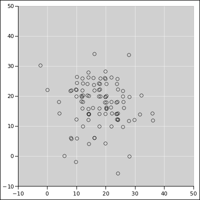
Figure ‍20: Binomial Distribution : Diaspogram		Figure ‍21: Binomial Distribution : XY Scatter Plot

3 References

1.

John Denker,
“spreadsheet demonstrating multi-parameter least-squares fitting using nonlinear basis functions”
./linear-regression.xls

2.

John Denker,
“Single- and Multi-Variable Data Analysis”
www.av8n.com/physics/linear-least-squares.htm

3.

Discussion of gnumeric bug #682734
https://bugzilla.gnome.org/show_bug.cgi?id=682734

4.

John Denker,
“spreadsheet for plotting arrowheads in data space”
./arrowheads.xls

5.

John Denker,
“Electric Charge and Potential: Spreadsheets for solving Laplace’s equation”
www.av8n.com/physics/laplace.htm

6.

John Denker,
“spreadsheet for calculating probabilities for two dice”
./dice.xls

7.

John Denker,
“spreadsheet for calculating probability distributions”
./histograms.xls

8.

John Denker,
“Tack Tossing : An Exercise in Probability”
www.av8n.com/physics/tack-tossing.htm