|
| |
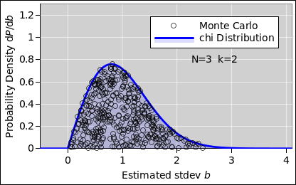
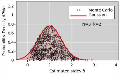
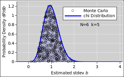
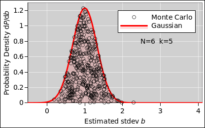
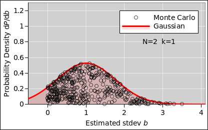
| Figure 1: Estimating the Standard Deviation | Figure 2: Estimating the Standard Deviation (Wrong) | |
Suppose there is a Gaussian probability distribution of the form A±B, where the nominal value A and the standard deviation B are not known. We designate that as our population. We do an experiment. Each run of the experiment produces a sample consisting of N data points, drawn from the population, and the task is to use that to estimate A and B.
For today, let’s concentrate on B. For simplicity, let’s anticipate that we will discover that B=1. However, we did not know that when doing the experiments; the point of the experiments was to find that out.
We assign 400 different students to do the experiment, one run per student. Let b denote the student’s estimate of B. We collect data from all the students, and do some meta-analysis.
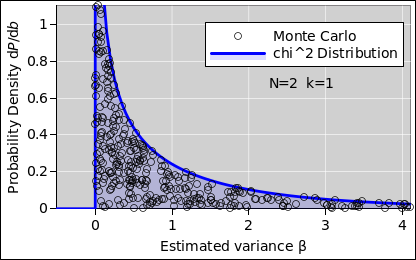
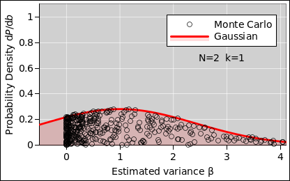
Let’s start with a sample-size of N=2 data points per run, as shown in figure 1. The first thing to notice is that the distribution of b-values is not Gaussian. It’s not even close, as you can see by comparing to figure 2, which is a Gaussian with the same mean and standard deviation.
Another thing to notice is that a substantial number of students obtained b-values that disagree with the true B-value by 90% or more, in one direction or the other. The students have not done anything wrong; the problem is purely statistical. The sample produces a noisy estimate of the properties of the population.
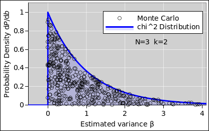
The situation is only marginally better with N=3 data points, as shown in figure 3. The sample is still a very noisy estimator.
By the time we get to N=6 data points per run, the distribution is beginning to look more-or-less Gaussian, but it’s still rather noisy.
Let’s look at an all-too-common formula for using the sample data to estimate the standard deviation of the population:
| (1) |
That shows up in lots of places, including e.g. Baird equation 2.9, where it is touted as the "best estimate". It is baked into the stdev() function in every spreadsheet I’ve ever seen.
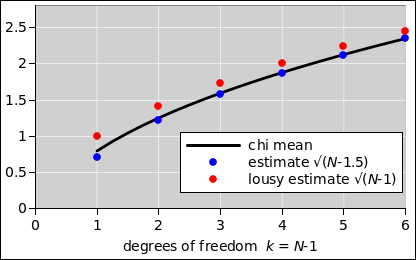
In particular, consider the factor of √(N−1) that appears in the denominator. Contrary to what is nearly-universally claimed, √(N−1) does not produce an unbiased or optimal estimator for the standard deviation of the parent population.1 It turns out that equation 2 is vastly better across the whole range, and even that’s not perfect for small N, as you can see from figure 7.
| (2) |
Here’s something that works even better:
| (3) |
where the successive means of the χ-distribution are:
| (4) |
where the simple expression on the last line is accurate within half a percent for all k>3.
There shouldn’t be any big mystery about this. The properties of the χ-distribution have been understood for quite a while now; see reference 1.
Now let’s suppose that after collecting data from all the students, rather than averaging their estimated standard deviations using a simple arithmetic average, we decide to take the root-mean-square (RMS) average instead. Depending on details, that might or might not be a smart thing to do. Let’s at least explore the possibility.
More-or-less equivalently, suppose that rather than paying attention to b, i.e. each student’s estimate of the standard deviation, we decide to pay attention to β, i.e. each student’s estimate of the variance, b2.
Now it turns out that the unbiased estimator for the variance is rather simple. The denominator is a factor of k i.e. N−1.
| (5) |
Let’s be clear: Even though the factor of √(N−1) is wrong in equation 1, the factor of (N−1) is correct in equation 5. The best estimate for b2 is not the square of the best estimate for b. Taking the average does not commute with taking the square root. Life can be quite nonlinear sometimes.
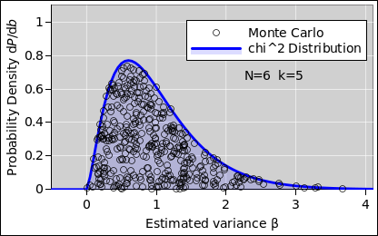
We can quantify this by using the chi-squared distribution (reference 2). It is famous, and textbooks give it far more attention than the chi distribution that we used in section 1. Sometimes it’s what you want – but sometimes it isn’t. It has some peculiar properties, as we now discuss.
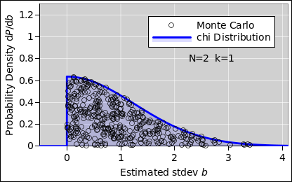
As you can see in figure 8, for N=2 (k=1), there is a more-than-astronomical chance that any given student will obtain a small variance. The estimator in equation 5 may be unbiased, but it’s still a very noisy estimator. Also, the distribution is very non-Gaussian, as you can see by comparing to figure 9, which is a Gaussian with the same mean and standard deviation.
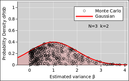
For N=3 (k=2), the situation is better, insofar as the probability density is at finite, but the distribution is still rather peculiar, as you can see in figure 10.
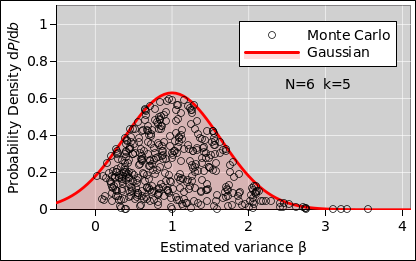
Even for N=6 (k=5), the distribution is markedly non-Gaussian, as you can see in figure 12.
Also keep in mind that the central limit theorem is not magic, and it does not solve all the world’s problems. Averaging a few points is not guaranteed to produce something close to Gaussian, as you can see in figure 13. The mean and standard deviation are correct, but the shape of the curve is wrong. It assigns far too much probability to small values of β, and even assigns nonzero probability to some negative values of β, which is absurd. Meanwhile, it assigns far too little probability to large values of β.