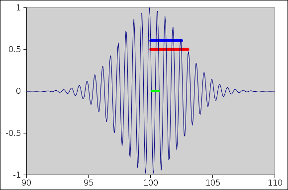
Figure 1: Wave Packet
The main goal here is to understand the difference between a hot electron and a cold, fast-moving electron.
However, before we can even approach the idea of a thermal wave packet, we need to review a few things about a plain old nonthermal wave packet.
A snapshot of a wave packet is shown in Figure 1. The snapshot was taken just as the wave packet crossed the location x=100. Actually the x-position doesn’t matter; today it suffices to look at the Δx values, so the absolute location drops out.
You can see that the dominant wavelength in the packet is about 0.6, as shown by the small green bar in the middle of the figure. This is what most people would think of as “the” wavelength. This corresponds to a nominal k value of k=10. From this we can calculate:
| (1) |
Meanwhile ... there is another length-scale to consider, namely the width of the envelope of the wave packet. The full width at half maximum (FWHM) is about 6. The half width at half maximum (HWHM) is about 3, as shown by the red bar in the figure. In fact the envelope was constructed to be a Gaussian with standard deviation of 2.5 units, as shown by the blue bar in the figure. The standard deviation is longer than the wavelength by a factor of 4.
If we take the Fourier transform, it tells us that a better description of the wavenumber is k = 10 ± 0.2. That is, we have about 0.2 units of spread in k-space. (This upholds the simple rule σx σk = 1/2.)
It must be emphasized that the wavefunction we are discussing here, as shown in figure 1, is non-thermal. It is a quantum state, a pure state, and as such has zero entropy and no temperature at all. In some sense it “looks like” it has zero temperature, but actually at this point in the discussion we cannot even define temperature. Usually temperature is T : = ∂ E/∂ S at constant V, but since every state we have constructed so far has zero entropy, the denominator of that expression doesn’t make sense. So for the moment, temperature is undefined and undefinable.
It is worth noting how this wavefunction behaves under a Galilean change of velocity. The dominant wavenumber k is changed, but the width σk is not changed. That’s because all the wavenumbers are changed by the same amount; the object shown in figure 1 undergoes a rigid shift in k-space.
Simplest reliable way to connect quantum mechanics with thermodynamics is via density matrices. See reference 1 for a discussion of how to calculate a density matrix, and how to calculate entropy in terms of the density matrix.
Notice in particular the great power of the density matrix: Whereas a quantum state vector |a⟩ represents a microstate, a suitable density matrix ρ can fully represent a macrostate.
A fancier and less-widely-known way to connect quantum mechanics with thermodynamics is via the “path integral” formulation, as discussed in reference 2.
As the temperature gets colder, the spread in k-space gets smaller, which means the spread in position-space gets larger. That’s right: cold wave packets are larger in size than hot wave packets. This is the opposite of what you would expect if you thought the size was due to thermal agitation. A bag of ideal gas gets smaller if you cool it down (subject to constant external pressure), but the individual wave packets get bigger.
Let’s look at some examples of states and density matrices. We choose a one-dimensional particle, and use the wavenumber basis. Let’s restrict attention to the seven 1k-values {−3, −2, −1, 0, 1, 2, 3}. For each basis state i, the energy is Ei = ki2.
| 1. Here is the density matrix for the ground state. It has E=0 and S=0. | 2. Here is the density matrix for a plane wave moving slowly to the right: It has E=1 and S=0. |
|
|
| 3. Here is the density matrix for a plane wave moving more quickly to the right: It has E=4 and S=0. |
|
| 4. Here is a low-energy standing wave. It has E=1 and S=0. It is not one of our basis states, but it is a stationary state, a pure state, a zero-entropy state, corresponding to the state vector |0, 0, R, 0, R, 0, 0⟩, where R := √½. | 5. Here is a higher-energy standing wave. It has E=4 and S=0. It is not one of our basis states, but it is a stationary state, a pure state, a zero-entropy state, corresponding to the state vector |0, R, 0, 0, 0, R, 0⟩. |
|
|
| 6. Here is a more complicated standing wave. It has E=0.5 and S=0. It is neither a basis state nor a stationary state, but it is a pure state, i.e. a zero-entropy state, corresponding to the state vector |0, 0, ½, R, ½, 0, 0⟩, where R := √½. | 7. Here is a running wave packet. It has E=4.5 and S=0. It is neither a basis state nor a stationary state, but it is a pure state, i.e. a zero-entropy state, corresponding to the state vector |0, 0, 0, 0, ½, R, ½⟩, where R := √½. It has the same average momentum as example 3, and the same spread in momentum-space as example 6. |
|
|
| 8. Here is a yet more complicated standing wave. It has E=1 and S=0. It is neither a basis state nor a stationary state, but it is a pure state, i.e. a zero-entropy state, corresponding to the state vector |0, 1/4, 1/2, Q, 1/2, 1/4, 0⟩, where Q := √6/16. |
|
| Up to this point, everything has been non-thermal. All the states have been pure states. |
| Let’s now consider thermal mixtures. |
| 9. First, though, let’s look once more at the density matrix for the ground state, the same one that we see in example 1, since it fits in both the thermal and non-thermal categories. It has E=0 and S=0. | 10. Here is the density matrix for a particle moving slowly to the right. It is the same as example 2. It has E=1 and S=0. |
|
|
| 11. Here is our first thermal state. It has E=0.5 and S=1.5 bit. It could be formed from example 6 by washing out the off-diagonal elements, as would happen if something perturbed the phases of the various contributions to the mixture. |
|
| 12. Here is a higher-lying thermal state. It could be formed from example 8 by washing out the off-diagonal elements. It has E=1 and S=2.03 bits. |
|
Let’s stop now and savor what has been accomplished. The sequence of states example 9, example 11, and example 12 can be seen as a sequence with progressively higher energy, progressively higher entropy, and progressively higher temperature. These three examples are only approximately thermal, because the microstate probabilities only approximately conform to the Boltzmann distribution, but they are good enough to make the points that need to be made. (They stand in contrast to things like example 4 and example 5, which are wildly nonthermal, because the low-energy microstates are wildly underpopulated relative to a Boltzmann distribution.)
In particular, example 10 has the same temperature as example 9, since the two states differ only by a Galilean transformation, i.e. a change in the velocity of the observer. In fact we assign T=0 to both states.
Now the interesting thing is that example 12 has the same energy as example 10. So we have accomplished what we set out to do: We have a no-nonsense way of understanding the difference between two states of the same energy, one of which is cold and fast, while the other is warm and slow. We can quantify the difference in terms of the entropy.
There are some follow-up points that need to be made:
The running wave in figure 1 has spread but zero entropy, and is therefore in the same family as example 7.
You could construct a hand-wavy derivation of some sort of “thermal wave-packet size” by setting p2/(2m) equal to (D/2) kT ... but this would be slightly different from the official thermal de Broglie length. It would be off by a factor of 2 π, and perhaps more interestingly it would be off by a factor of D, where D is the dimensionality of space (D=3 usually).
There are good reasons why the thermal de Broglie length is defined the way it is. Deep reasons, connected to the uttermost foundations of statistical mechanics. For example, in the high-temperature limit the partition function for a particle in a box reduces to a remarkably simple expression:
| Z = |
| (2) |
where V is the volume of the box and Λ is the thermal de Broglie length. For a derivation of this, see reference 1.
Physical example: Spin waves observed at low temperatures and not otherwise. Need to cite Bashkin. Need to cite reference 3 and reference 4.
This tremendously advances our understanding of physics, because it lets us get our hands on the boundary between quantum mechanics and the classical approximation. If the scattering is classical at high temperatures and quantum-mechanical at low temperatures, we can sit at an intermediate temperature and see what happens. In fact we see weak spin waves, because the particles are partially distinguishable and partly not.
The thermal de Broglie length plays an interesting role during the collision between two nominally-identical particles. See reference 5.