Loosely speaking, sound is a mechanical disturbance in some medium.
There is an interplay between inertia (involving the density of the
medium) and a restoring force (involving the elastic properties of the
medium, i.e. pressure and/or shear stress). Coming up with a more
precise definition would not be worth the trouble, for reasons
discussed in reference 1.
The medium can be solid, liquid, gaseous, or whatever.
The disturbance can be longitudinal or transverse, although in liquids
and especially in gases a transverse sound wave is usually so grossly
overdamped as to be not worth worrying about.
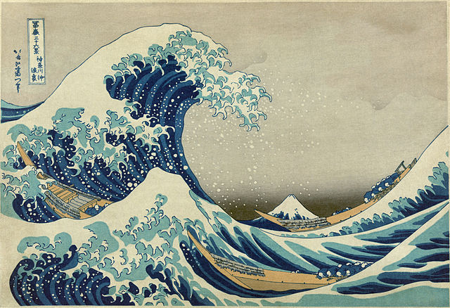
Gravity waves on the surface of the ocean are generally not considered
sound waves. Also capillary waves on the surface are generally not
considered sound waves, although it is hard to define “sound” in
such a way as to exclude them. In contrast, solids have surface
acoustic waves which behave differently from acoustic waves in the
bulk.
Acoustic wave is synonymous with sound wave.
Sound is not limited to the range of human hearing. The dictionary
defines ultrasound to be a form of sound. Cats can hear sounds up to
70 kHz or thereabouts. Dolphins can hear sounds up to 150 kHz or
thereabouts.
We define a wave to be something that exists as the solution to a wave
equation. It is best to focus attention on the wave equation rather
than the wave itself. See section 3 for a discussion
of wave equations.
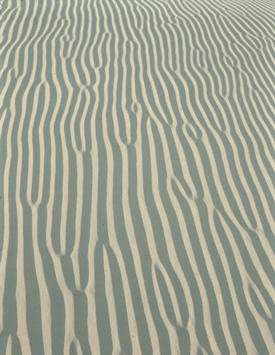
To say the same thing the other way: You cannot tell whether something
is a wave or not just by looking at it, if you don’t understand the
physics that produced it. In particular, the sand ripples in figure 3 are a wave, whereas the ridges and furrows in figure 6 are not, although you could never tell by looking
at the pictures. Sometimes a movie will reveal the physics in
situations where a snapshot would not, but even a movie is not
necessarily sufficient, e.g. in the case of a standing wave.
Just because it is repetitive does not make it a wave, as we see from
the examples in section 1.2.
On the other side of the same coin, a wave does not need to be
repetitive. It does not need to have any zero-crossings. Example: A
single pulse propagating along a string. The pulse in figure 7 repeats every few seconds (to make it easier to
see), but you can imagine a pulse that occurs only once.
Sometimes a wave can be partially repetitive and partially not. It
can have a finite number of zero crossings. Example: A carrier
modulated by an envelope, as in figure 8.
Again, the central idea is that the wavefunction is a solution to a
wave equation. You may be accustomed to solving an equation to find a
number, but you can perfectly well solve an equation to find a
function. A function is more complicated than a scalar, just as a
movie is more complicated than a poster. However, it is possible to
go shopping for a movie instead of a poster. Most functions are not
solutions to the wave equations, just as most movies are not the one
you want to buy.
Here are some examples of solving an equation to find a function:
An exponential function of time is a solution to the
equation that says the number of bacteria doubles every hour.
A parabolic function is a solution to the equations of motion
for a particle moving in a uniform gravitational field.
An elliptical function is the solution to the equations of
motion for a planet going around the sun.
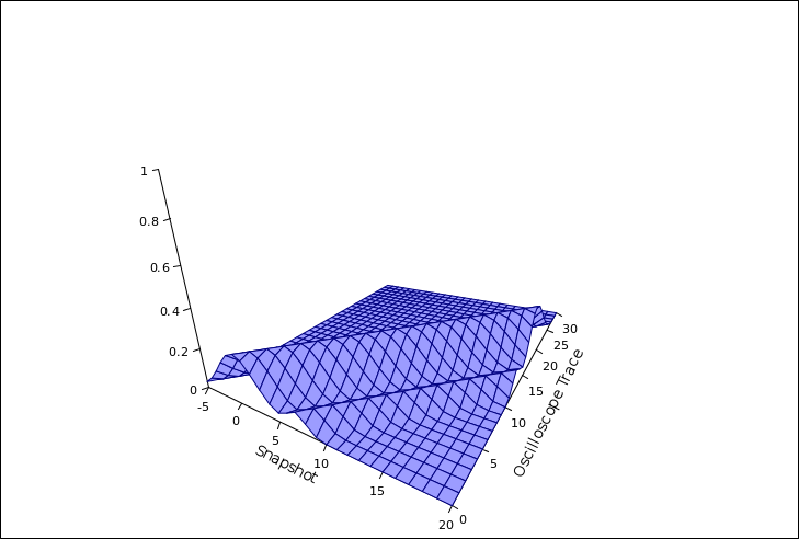
Figure 9 is a three-dimensional plot, but each of the
three dimensions represents something different. The spatial
x-coordinate increasas from the left to the lower right. Time
increases from the front to the right rear. The ordinate of the wave
function is more-or-less vertical up the page.
If you look along the axis where it says “snapshot”, that
corresponds to taking a snapshot of what the wave looks like, across
all positions, along a contour of constant time=0. The wave is moving
left-to-right, although you cannot tell that from a single snapshot.
At time=0, the main peak is centered at position=0, and there is a
subsidiary peak at position=7.
If you look along the other axis, where it says “oscilloscope
trace”, that corresponds to sitting at a fixed location, namely
position=20, and using an oscilloscope to observe what the
wavefunction does at that one location, as a function of time. The
subsidiary peak arrives at time=13. Then the main peak arrives at
time=20.
A wave does not need to propagate. There are such things as standing
waves. For a linear medium, we can describe the situation as follows:
The standing wave has a definite shape as function of position
(independent of time). It just sits there and gets bigger and smaller
in proportion to a function of time (independent of position). So
there is a separation of variables. Also, you can think of a standing
wave as the superposition of a running wave with an equal-and-opposite
running wave.
Examples include:
Standing waves on a violin string. (S) (AH)
Standing waves in a cylindrical bore, such as a flute, clarinet,
et cetera. (S)
Acoustical or electromagnetic standing waves in a rectangular
cavity. (S)
Acoustical or electromagnetic standing waves in a
non-rectangular cavity.
Standing waves on the surface of a non-rectangular swimming pool.
Atomic wavefunctions such as |1s⟩ and |2pz⟩, as discussed in
reference 2. (AH!)
Standing waves on an ordinary (non-rectangular) drumhead.
Standing waves in a conical bore such as an oboe, saxophone, et cetera.
Standing waves on a chain with non-uniform tension. (This can
easily happen if the chain’s own weight makes a nontrivial
contribution to the tension.) (AH)
The items marked (S) exhibit a more-or-less sinusoidal pattern as a
function of position, whereas all the others don’t. The items marked
(AH) are perceptibly anharmonic (i.e. nonlinear) at readily-achievable
amplitudes.
In all cases, the criterion for a wave to be a standing wave is
that it does not transport energy from place to place. For example,
consider a nice simple sinusoidal standing wave on a string. The
ordinate of the wavefunction is the height of the wave, denoted
ϕ, which is implicitly a function of x and t. At each
point x, the ordinate is ϕ=sin(ωt). The
corresponding velocity is ϕ·=ωcos(ωt). The
potential energy is proportional to ϕ2 and the kinetic energy
is proportional to ϕ·2. The constants of
proportionality are such that the total energy is proportional to
sin2 + cos2 ... which is a constant. There is no energy flowing
from place to place.
In section 2 we defined a wave as something that is a
solution to a wave equation. That leaves us with the obvious
question, what is a wave equation?
There are lots of different wave equations, some of which are more
complicated than others. In particular, the wave equation for an
electromagnetic wave in a waveguide is more complicated than for an
electromagnetic wave in free space. In quantum mechanics, the wave
equation – i.e. the Schrödinger equation – has complexities all
its own.
Here are the key things that all these have in common: The equation
involves at least two variables: one timelike variable and one
spacelike variable (which may belong to a very strange abstract
space). It is possible, at least in principle, to have a solution
that moves from an initial location at one time to a nearby location
at a later time, maintaining the same shape, or at least almost the
same shape. This is called a running-wave solution.
To repeat: To qualify as a wave equation, it must have some
running-wave solutions.
On the other hand, as mentioned in section 2.3, we do not
require that all solutions be running waves. Very commonly it is
possible to combine running waves so as to make a standing wave, i.e.
a solution that does not propagate from place to place. This does not
disqualify the equation from being a wave equation. Similarly, the
standing wave counts as a wave – because it is a solution to a wave
equation – even though you couldn’t necessarily ascertain this just
by looking at a snapshot of the solution. On the other hand, if an
equation has only non-propagating solutions, then it probably
shouldn’t be considered a wave equation.
Tangential remark: It is fairly common for the solutions of an
equation to have a different symmetry from the equation itself. For
example, a roulette wheel has N=37 or N=38 slots, each of which is
supposed to have the same size, same depth, and same probability.
This gives us an equation with N-fold symmetry. However, on any
particular play of the game, the marble winds up in only one of the
slots. The ensemble of all possible outcomes is symmetrical, but any
given outcome is not symmetrical. I mention this to support the idea
that it is OK for the wave equation to have standing-wave solutions as
well as running-wave solutions.
See reference 3. This is the classic video from 55 years ago.
Note that even today, the torsion-wave demonstration apparatus is
sometimes called a Shive machine.
For reasons discussed in reference 4, I disagree with the
way he uses the words “cause” and “effect”, but that is
unimportant and tangential to the points he is making.
A shorter video showing just the reflection situation is
reference 5.
In both of these demos, they missed a trick insofar as they kept the
torsional spring constant the same and varied only the moment of
inertia of the ribs. Therefore the wave speed changes along
with the impedance. Students can’t tell from the demo whether the
important thing is the impedance or the speed. Those who know about
Snell’s law will be fixated on the speed.
Suggestion: The smart thing would be to change the torsional stiffness
in proportion to the moment of inertia, so that the wave speed stays
the same even as the impedance changes. I have not yet found video of
that.
On the other side of the same coin, figure 10 shows
what happens when a wave propagates from one medium to another. On
the left side of the diagram, the medium is polyester rope. On the
right side of the diagram, the medium is brass chain. However, I
arranged things so that the impedance is the same, so there is no
reflection.
The problem with using a rope (or chain) instead of a torsion
apparatus is that the wave speed is inconveniently high. A the
acceleration of gravity being what it is, the rope will always be
under a fair bit of tension, just to support its own weight. This
gives rise to a minimum wave speed. You can increase the speed
by increasing the tension. There are ways of reducing the tension,
e.g. by supporting some of the weight of the rope in the middle, but
this is not super-convenient. Unless the rope is very long, the high
speed makes hard to visualize what is going on. You can alleviate the
problem somewhat by viewing the rope almost end-on, so that the
distance along the rope is foreshortened. I used a fair amount of
foreshortening in figure 10.
5 Dispersion, Dissipation, Nonlinearity, and Shocks
In the simplest case, all waves in a given medium travel at the same
speed. However, this is definitely not always the case.
You can easily have a situation where a large-amplitude wave travels
at a different speed from a small-amplitude wave. This is called
nonlinearity. This is quite common for water waves in a shallow
channel. In some cases this can lead to a tidal bore, which is
a kind of shock (aka shock wave). (Experts tend to call such things
shocks, rather than shock waves.)
It is also possible to have a situation where a long-wavelength wave
travels at a different speed from a short-wavelength wave. This is
very common for waves on the surface of deep water. There’s actually
a minimum in the wave speed; shorter waves are faster (due to surface
tension) and longer waves are also faster (due to gravity). You may
be aware that a tsunami is a long-wavelength wave, moving at
tremendous speed, commonly 800 to 1000 km per hour, almost the speed
of sound in air. It is well known that the ordinary waves you see at
the beach (wavelength on the order of meters) do not travel nearly so
fast.
Last but not least, it must be pointed out that the wave equation in
polar coordinates is dispersive, even in situations where plane waves
in the same medium would be non-dispersive. This has tremendous
practical consequences. For one thing, you may have notices that an
explosion up close makes a short “snap” noise, whereas an explosion
farther away makes a “boom” noise.
Part of the difference is explained by dispersion; different
frequency components travel at different speeds.
Part of the difference is explained by absorption; shorter
wavelengths die out more quickly.
It is also worth noting that in the real world, a wave loses energy as
it moves along. For example, a sound wave in air can lose energy do
to viscosity, and also due to thermal conductivity. At the peaks of
the sound pressure field, the air is always slightly hotter than in
the troughs, so there can be losses due to thermal conductivity,
although this effect is small when the wavelength is long. Similarly,
compressing and decompressing the air dissipates energy via bulk
viscosity. There can be vastly greater dissipation at boundaries, via
shear viscosity. (This is how “acoustical tile” works.)
In the typical introductory course, nobody worries about dispersion,
dissipation, nonlinearity, or shocks. However, such things are worth
mentioning at least once, in hopes of cutting down on the number of
misconceptions. It would be a misconception to think that all waves
are linear, non-dispersive, and/or non-dissipative.
The Music Science site at UNSW is awesome. It contains an enormous
amount of material, most of it very readable, with very high levels of
technical accuracy. See reference 6.
Reference 7 has a collection of high-quality animations. I
particularly like the longitudinal wave animation, because it seems
physically correct for a lattice of regularly-space particles. It
doesn’t pretend to be something it isn’t.
Reference 8 is well worth a bookmark. There are dozens
of pages, each with several animations. The first few are quite
basic.
On the first page, there is an adorable animation of stick
figures “doing the wave”.
However, I don’t like the "dictionary definition". It rules out
standing waves. I know a lot of chemists who would get cranky if you
told them that s-waves and p-waves are not waves.
I also don’t like the diagrams that look like molecular dynamics
simulations of particles in a gas (on the first page and elsewhere).
They are fake data pretending to be something more. (I usually don’t
object to data that is obviously fake.) You can’t have a sound
wave in a gas if the gas particles themselves aren’t moving. These
animations are just begging to be misinterpreted.
On the second page, there is an animation to help explain the
relationship between a snapshot and an oscilloscope trace.
On later pages, there are the usual animations of reflection
from an impedance mismatch ... although I prefer video of real
experiments, whenever possible, rather than simulations.
After the first few pages, things rapidly get more
sophisticated.