Turbid User’s Guide
John S. Denker
ABSTRACT: We discuss how to configure and use turbid, which
is a Hardware Random Number Generator (HRNG), also called a True
Random Generator (TRNG). It is suitable for a wide range of
applications, from the simplest benign applications to the most
demanding high-stakes adversarial applications, including cryptography
and gaming. It relies on a combination of physical process and
cryptological algorithms, rather than either of those separately. It
harvests randomness from physical processes, and uses that randomness
efficiently. The hash saturation principle is used to distill
the data, so that the output is virtually 100% random for all
practical purposes. This is calculated based on physical properties
of the inputs, not merely estimated by looking at the statistics of
the outputs. In contrast to a Pseudo-Random Generator, it has no
internal state to worry about. In particular, we describe a low-cost
high-performance implementation, using the computer’s audio I/O
system.
Other keywords: TRNG, HRNG, hardware random number generator, uniform
hash, unbiased coin flip.
* Contents
1 Emergency Operations
If you need some randomness right away, take a look at the suggestions
at the beginning of reference 1.
2 Turbid: Goals and Non-Goals
2.1 Basics
The basic objective of turbid is to provide a supply of
randomly-generated numbers, with quality and quantity suitable for a
wide range of applications, including some very demanding
applications. Some specific applications are discussed in
reference 2. Quality requires, among other things,
defending against various possible attacks. Some well-known attacks
are discussed in reference 2. Some background and
theoretical ideas are outlined in section 5 and
developed more fully in reference 2.
Right now, in this section, we give a broad outline of what is
possible and what is not possible.
So far, we have analyzed the HRNG mainly in terms of the density of
adamance, denoted by ρ. We choose a criterion ρmin very
close to 100%, and then build a generator that produces ρ >
ρmin. We are not pretending to achieve ρ = 100% exactly.
2.2 Tradeoffs
Here are some of the criteria on which a random generator can be
judged:
- High-quality outputs, exceedingly resistant to outside attack,
i.e. cryptanalytic attack.
- Efficient use of the randomness coming from the raw inputs.
- Efficient use of CPU cycles.
- Ability to meet short-term peak demand.
- Rapid recovery from compromise, including inside attack,
i.e. capture of the internal state.
These criteria conflict in complex ways:
These conflicts and tradeoffs leave us with more questions than
answers. There are as-yet unanswered questions about the threat
model, the cost of CPU cycles, the cost of obtaining raw randomness
from physical processes, et cetera. The answers will vary wildly from
platform to platform.
3 Installing the Ingredients
- A typical Linux distribution comes with ALSA. It is usually
pre-installed, but if not, installation is easy. Install ALSA,
including the drivers, utilities, and development libraries
(libasound2-dev). See reference 3 for details on what
ALSA provides.
The current turbid code is compiled against version 1.0.25 of the
libraries. Slightly older versions should be satisfactory; much
older versions are not. If you are compiling from source, you might
want to apply the patch in turbid/src/excl.patch, so that the mixer
device can be opened in “exclusive” mode. To do that, cd to
the directory in which you unpacked the turbid and alsa
packages, and then incant something like patch -p1 <
turbid/src/excl.patch. Then configure, make, and install the ALSA
stuff (drivers, libraries, utilities). If you have never run ALSA on
your system, you will need to run snddevices once. It may
take some fussing to get the proper entries to describe your
soundcard in /etc/modules.conf. Install the utils/alsasound
script in /etc/rc.d/init.d/.
- Test the sound system. Verify that you can play a generic .wav
file using aplay. Then verify that you can record a signal
and play it back. This step is especially helpful if you are having
problems, because it tells you whether the problems are specific to
turbid or not.
        :; sox -r 48000 -b 32 -t alsa hw:0  -c 1 noise.wav  trim .1 3
or
        :; arecord -D hw:0 --disable-softvol -f S32_LE -r 48000 -V mono -d 3 noise.wav
then
        :; aplay noise.wav
        :; od -t x4 noise.wav
- Compile turbid. This should require nothing more than
untarring the distribution and typing make in the
turbid/src directory.
- You don’t need to be root in order to compile and test
turbid. If you want to run turbid as non-root, make
dirs to create the needed directories, as follows:
If turbid runs as non-root, it will open its output FIFOs in your
$HOME/dev/ directory, look for its control files in your
$HOME/etc/turbid/ directory, and scribble a .pid file in your
$HOME/var/run/ directory.
In contrast, if turbid runs as root, it will use the system
/dev/ and /etc/turbid/ /var/run/ directories.
- Test and calibrate the audio hardware as discussed in the next
section.
- Send me <jsd@av8n.com> the results of the configuration, including
alsamixer’s .ctl file, and turbid’s values for Rout,
Rin, gVout, gVin, and bandwidth. I will
add it to the distribution, so that others may use that brand of
cards without having fuss with calibration.
- You can (if you want) become root and do a make install.
- If you want turbid to be started and stopped automatically
according to the system runlevel, you need to install a few things by
hand. There is a file turbid/src/init.d/turbid which you can
use as a model for something to put in to /etc/rc.d/init.d/
(but don’t forget to edit the options, according to the calibration,
as described below). This is not installed automatically; you have
to do it by hand. Similarly you need to install by hand the symlinks
in /etc/rc.d/rc?.d/.
4 Configuration and Calibration
Note: You can skip this section if you’ve been given a suitable
turbid.tbd configuration file and mixer configuration
(.ctl) file.
Configuration is important. It is remarkably easy to mis-configure a
soundcard in such a way that it produces much less randomness than it
otherwise would. This section outlines the general procedure; see
appendix B for details on specific soundcards.
Terminology: we use the term soundcard loosely, to apply
not just to card-shaped objects per se, but also to audio I/O
subsystems embedded on the mainboard, USB dongles, external pods, et
cetera.
4.1 Configuring Audio Output
-
You will need the following supplies. Most of this
stuff can be borrowed. For example, if things go well, the
headphones, the music player, and the voltmeter are only needed for
a few minutes.
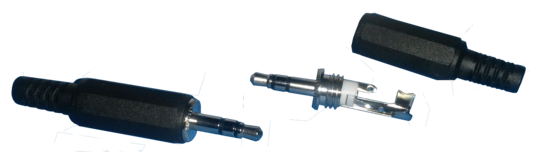
- Two 1/8” stereo audio plugs. They have to be stereo, even if
you plan on using only one channel. These are also called 3.5 mm
plugs, although 1/8” is less than 3.2 mm. (If you found something
that was actually 3.5 mm, it wouldn’t fit in the jack.) Figure 1 shows one with with its backshell removed, and
another with its backshell in place.
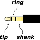
See figure 4 and table 1 for the
layout of a standard stereo connector.
- Alligator clips. Get a package with assorted colors. You want
ones with nice small clips. A length of 1 foot (30 cm) is fine.
- Multimeter. You want one that will read (at least) DC voltage,
AC voltage, and resistance.
- Matrix board, also known as “solderless breadboard”. See
figure 2. You may think you can get by without this,
but things will go easier if you use one. A very small one is
sufficient for present purposes.
- Some sort of shield box, of a size to fit over the matrix board
and the circuits you have built on it, to shield them from
interference. See item 27 for the next level of detail on
this.
- Resistors. You can get a “party pack” containing 500
resistors of various values from 1 ohm to 10 Megohm. A power rating
of 1/4 watt or even 1/8 watt is sufficient.
- Headphones. (You could perhaps use loudspeakers instead of
headphones, but for simplicity and consistency this document will
speak in terms of headphones.)
- A smartphone, a portable music player, or something similar
to use as a signal generator.
- An audio cable, for temporarily hooking the aforementioned
player to the computer you are configuring to run turbid.
-
Note: At any time, you can run turbid show
args to see what it thinks it is doing. For example, the card
line tells you what ALSA device it wants to use.
Also note: When it starts up, turbid automatically takes commands
from the configuration file turbid.tbd if it exists in the
working directory. Other configuration files can be invoked on the
command line using the “@” sign, as in turbid @foo.tbd for
example.
-
Choose an output port. The first choice is
Line-Out, the second choice is Headphone-Out, and a distant third is
Speaker-Out.
-
Configure turbid to use the proper card. See
section 6.3 for guidelines on choosing a suitable card.
If you’re lucky, the default ALSA device (hw:0,0) corresponds to the
proper card. Otherwise you will have to specify card ... on
the turbid command line. Putting it into the turbid.tbd file is a
convenient way to do this.
The choice of card cannot be changed while turbid is running, so to
experiment you need to stop turbid and restart it in the new
configuration.
-
Plug your headphones into the chosen output port, then
fire up turbid sine .2 and see what happens.
- You may need to adjust the volume using alsamixer.
- You can also adjust the sine amplitude on the turbid gui, but
you shouldn’t set it too much below 0.1 or above 1.
- There may also be a physical mute button, volume controls,
etc. on your keyboard. With any luck these functions are not
separate from the corresponding ALSA mixer functions, but if they are,
you will have to be careful – from now on – to keep them properly
configured.
If that doesn’t work, some investigation is required. The command
aplay -L (capital letter L) and/or aplay -l (lowercase
letter l) to see what audio devices are available. If there are none,
or only trivial devices such as “null”, you might try bestowing
membership in the “audio” group to the user who will be running
turbid. If the card you want to use is not visible, check that the
hardware is installed (lspci -v -v or lsusb -v -v).
Then check that the appropriate drivers are loaded.
- In the output of aplay -L you might see something
like this:
      hw:CARD=Intel,DEV=0
          HDA Intel, CX20561 Analog
          Direct hardware device without any conversions
in which case you can invoke turbid card hw:CARD=Intel,DEV=0.
- In the output of aplay -l you might see something
like this:
        card 0: Intel [HDA Intel], device 1: CX20561 Digital [CX20561 Digital]
          Subdevices: 1/1
          Subdevice #0: subdevice #0
in which case you can invoke turbid card hw:0,1 where the zero is
the card number and the 1 is the device number on that card.
-
Plug one of your audio plugs into the jack
for the chosen port and leave it plugged in from now on, at all
times when turbid is running. That’s because there are situations
where plugging and unplugging causes the mixer settings to get
changed behind your back. This can lead to tremendous confusion.
The pulseaudio daemon is infamous for this, but there may be other
culprits.
If the plug gets unplugged, plug it back in and restart turbid
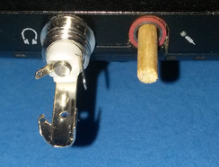 Figure 3
: Output Port Open-Circuited using an Audio Plug
-
We will calibrate one channel at a time. In theory
you could speed things up by working on multiple channels at once,
but there are an awful lot of things that could go wrong with
that. The examples that follow assume channel 0, i.e. the left
channel.
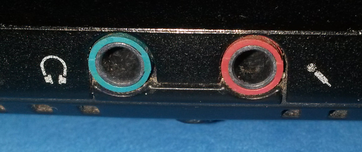
See figure 4 and table 1 for the
layout of a standard stereo connector.
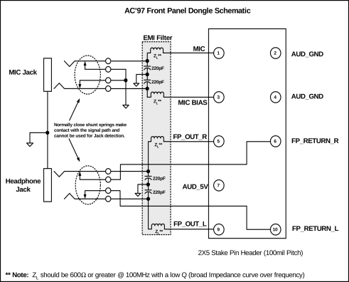
Beware that on a typical mono mic-input jack, the “ring” connection
is not an input at all, but instead a power output
(Vbias).
| name: | | tip | | ring | | shank | |
| name: | | tip | | ring | | sleeve | |
| channel: | | #0 | | #1 | | shield | |
| output usage: | | left | | right | | ground | |
| line-in usage: | | left | | right | | ground | |
| mic-in usage: | | left | | Vbias | | ground | |
Table 1: Audio Connector Properties
-
Using clips, temporarily connect headphones to the
chosen output signal. This is shown in figure 5. You
could have just plugged the microphone directly into the jack, but
remember we want the existing jack to stay plugged in.
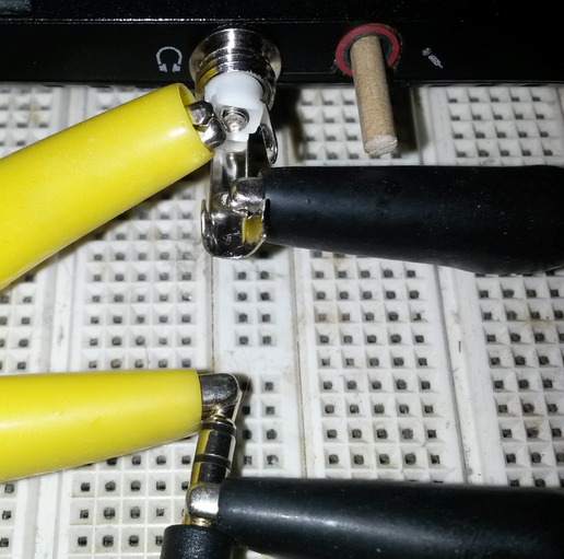 Figure 5
: Headphone Hooked Up Using Clips
-
Fire up turbid mixer "" sine .2 to invoke the
calibration feature. It plays a sine wave at 440 Hz (Concert A).
Debug things until you can hear this via the headphones.
Use alsamixer to adjust the output to some reasonable level.
You don’t want the output to clipped or otherwise distorted.
-
Once you have a reasonable mixer configuration,
save it to disk, as follows: Use turbid show args exit | grep
mixer-ctl to find what filename turbid wants to use for the
default mixer control file. Then use the command alsactl store
-f whatever.ctl to save the configuration to that file. (That’s not
a turbid command; alsactl a separate program, part of the
alsa package.)
If you want to use some other filename, that’s fine, but then you will
need to add the mixer some-other.ctl option to every turbid
invocation from now on. The turbid.tbd file is a convenient place
to put that sort of thing.
-
Disconnect the headphones. All critical measurements
should be made with the headphones disconnected. 1
-
Let’s calibrate the output conversion gain. The audio
plug should still be plugged in. It should look like figure 3. Fire up turbid sine .2, or whatever
amplitude you determined in item 9. Use a voltmeter to
measure the voltage of the chosen channel relative to the ground lug
on the audio plug. Use the “AC Volts” mode on the voltmeter.
You can do this using clips, but it’s probably quicker to just touch
the voltmeter probes to the correct lugs on the audio plug
Go to the Vopen page on the turbid gui, and enter the observed
voltage reading into the Vopen box. When you hit enter, this
will update the gain factor (gVout), and correspondingly update the
nominal sine amplitude. The sine amplitude should now be calibrated
in actual volts, and should remain so from now on.
Note: On this page, there is no need to enter anything into the gVout
box. The point of this page is to calculate gVout for you, when you
enter the Vopen reading.
Note: In all cases, when we talk about a measured voltage – output
voltage or input voltage – we mean RMS voltage (unless otherwise
stated). If you are using an oscilloscope or something else that
measures peak voltage, keep in in mind that the zero-to-peak
amplitude of a sine wave is 1.4 times the RMS value ... and the
peak-to-peak excursion is 2.8 times the RMS value.
-
Check for linearity, i.e. for the absence of
clipping. At an output level of 0.2 volts, clipping is unlikely, but
checking is easy and worth the trouble.
Procedure: Go to the turbid gui and change the sine amplitude up
and down. The output voltage, as observed on the voltmeter, should
track the nominal sine amplitude. If lowering the amplitude gives a
larger-than-expected output voltage, recalibrate at the lower
voltage. (Don’t go to such low voltages that you get into trouble
with noise, and/or with the limitations of the voltmeter.)
Find the largest voltage where things are still linear, then decrease
that by approximately a factor of two, and then make it a nice round
number. Use that as the “standard” sine amplitude setting from now
on. Go to the Vopen box and hit enter one more time.
Most soundcards can put out 1 volt RMS without distorting, so a
“standard” sine amplitude of 0.5 would not be surprising.
-
When you hit enter as described in
item 13, turbid should have written a oropoint line and
a gVout line to the terminal, i.e. to standard output.
You probably want to copy-and-paste these two lines into your
turbid.tbd file.
-
[Optional] Do a sanity check on the frequency
dependence. Measure the voltage at (say) 220 Hz, 440 Hz, and 880 Hz.
All readings should all be roughly the same. At some sufficiently
high frequency, the voltmeter will no longer be reliable.
As a point of reference, the venerable Fluke voltmeter I use for this
is rock solid up to 1 kHz. There is a 1-pole corner at 4 kHz. Above
roughly 30 kHz the bottom drops out. Remember, this step is
optional; if you are in a hurry you do not need to check your
voltmeter with anywhere this level of detail.
-
Let’s calibrate the output impedance. Switch to the
Vloaded page on the turbid gui. You can switch pages by clicking
on the named tabs, or by using the Control-PageDown and
Control-PageUp keys on the keyboard.
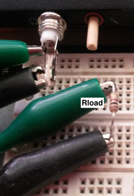
Hook up the circuit shown in figure 7. Choose a resistance
that will be small enough to decrease the voltage to roughly half of
the open-circuit voltage. An initial guess of 100 Ω is
reasonable. Measure the resistance using the multimeter. (Don’t rely
on the markings on the resistor, except possibly as a rough guide when
picking a resistor. For determining the actual resistance, the meter
is more accurate and more convenient.) Plug the ends of the nresistor
into two different rows in the matrix board, and then use clips to
hook it across the output.
Enter the resistance value into the Rload box on the gui.
Then – after you have entered the resistance – measure the
voltage across the output, on the lugs of the audio plug. Enter this
into the Vloaded box on the gui.
On this page, there is no need to enter anything into the Rout box or
the gVout box. The point of this page is to calculate Rout for you,
when you enter the Vloaded reading.
-
When you hit enter as described in
item 16, turbid should have written a oropoint line and a
Rout line to the terminal, i.e. to standard output.
You should probably copy-and-paste these two lines into your
turbid.tbd file. (This is in addition to the two lines from the
Vopen page.)
4.2 Choosing an Input Port
-
Choose an input port. On some machines, including
some laptops, you have only one possible input, namely
microphone-in. On other machines you have multiple possiblities, in
which case the following considerations should guide your choice:
- More sensitivity is good, more bandwidth is good, and multiple
channels is also good. Alas there is sometimes a tradeoff between
sensitivity and multiplicity, as discussed below.
- Microphone inputs are sometimes more sensitive than line-level
inputs.
- Microphone inputs are often mono. Beware of the following:
- On a mono Mic port, the tip is the actual input. In a stereo
situation this would be the left channel, but here it is the only
channel. Beware that very commonly the ring is an output,
namely a bias voltage for powering electret microphones. It is not
an input at all. The typical “soundblaster” product supplies a
+5V bias voltage through a 2.2kΩ resistor. However, you can’t
count on this; I’ve seen some laptops where the open-circuit voltage
is only 2.5 volts (again with a 2.2kΩ output impedance).
This is scary, because if you try to monitor the input in such a way
that the microphone bias voltage gets routed to a real stereo input,
it is entirely possible for the DC on the right channel to blow out
your speaker.
- Some soundcards allow you to make a “stereo” recording from a
mono Mic input. Hypothetically, it is conceivable that sometimes the
two channels have uncorrelated noise. However we have no way of
proving this, and no way of calibrating how much independent noise
there is. Therefore, in such a situation, it is safest to assume
that only one channel is usable as our source of unpredictability.
- I’ve seen some machines where the input port was configurable,
such that it was optionally mono Mic-in and optionally some sort
of stereo input.
At the chip level, most audio hardware these days is extremely
configurable. This includes low-level details such as the number of
input and output channels on each port. However, on most machines
it’s not obvious how make changes to the low-level configuration. It
may be that the hardware doesn’t support it, or the ALSA drivers
don’t support it, or I’m not smart enough to figure it out. If
anybody has good information on this, please let me know.
See also section H.
- If there is a tradeoff between more channels (stereo line-in)
and more sensitivity (mono Mic-in), then:
- Sometimes the line-level input is so insensitive as to be
essentially useless. In this case, the mono Mic input is the
correct choice.
- If the line-level input has some reasonable sensitivity, it is
unlikely that the Mic input is twice as good. In this case, the
stereo input is your best choice.
It may not be entirely obvious a priori what is your best is.
You may have to go through the calibration process on each input to
decide which provides the most randomness per unit time.
4.3 Configuring Full-Duplex Audio
Take a moment to think about the following issue: We want to set up
full-duplex audio. Full duplex means that the input signal is
independent of the output signal. Most likely, you will have to
fiddle with mixer settings (using alsamixer) to get this to
work. Presumably you already have the output working (section 4.1), so now we need to get the input working without
messing up the output.
This is trickier than it might seem, because recording engineers very
commonly want to monitor the signal that is being recorded, there is
sometimes a path within the mixer whereby the input signal can be
looped back to some output. This kind of loopback interferes with
what we are trying to do. This kind of mixer mis-configuration is
sometimes hard to detect. Note the contrast:
|
Recording engineers want to do input, with immediate
re-output via the mixer (hairpin).
|
|
We want to do output, with
immediate re-input via the calibration resistor network
(loopback).
|
Therefore, when configuring the input subsystem, the safest procedure
is to use a signal that comes from a second, separate system.
- The computer being configured to run turbid;
call this the turbid system.
- Something to produce a well-behaved test signal; call this the
signal generator system, or simply the player system. Your
options for this include:
- For some people, the simplest thing is to use a smartphone
or a portable music player. Download the audio file
(sine.wav), or create one from scratch using the
mkwav program (which is bundled with turbid). Download it
into your player. Set up the player app so it plays the file
over and over, since it would be very confusing if it stopped
playing and you didn’t notice.
- Another option is to find a laptop (not the turbid
system you are configuring) and use that as a signal generator.
You can either run turbidsine .2 to generate a signal, or play
the aforementioned audio file using aplay sine.wav.
So ... here’s the plan:
-
Set up the player system. Use the headphones to
listen to its output. Verify that it is at a reasonable level. Then
disconnect the headphones.
Note: Do not leave the headphones plugged in during the
measurements that follow, when the player output is connected to the
turbid input. In other words, do not use a “Y” splitter. That’s
for two reasons: - First of all, you run the risk of blowing out the right channel
of your speakers, if you bridge output to microphone-input to
speaker-input. As discussed in item 18, keep in mind that
the right channel of the microphone jack is not an input at all, it’s
a power output.
- Secondly, the headphones or speaker present an ill-characterized
load to the system, interfering with any attempt to make quantitative
measurements; see step 11.
-
Run the audio cable from the player system to the
chosen input port on the turbid system.
-
Fire up turbid sine .00001 and look at the Magnitude
box on the gui. If necessary, use alsamixer to configure the
recording-mode properties of the mixer so that turbid is receiving
a reasonable input signal. You don’t need to worry about exact signal
levels at this stage, but the following qualitative criteria should be
satisfied:
- Turbid should get a good-sized Magnitude reading when the
signal is connected.
- The reading should drop to a low level when the signal is
removed, e.g. by pausing the player, or by disconnecting
the audio cable at the player end (not at the turbid end).
- Clip the headphones to the output port, and verify that no
vestige of the signal is heard. That is to say, we want i.e. no
“record monitor” behavior.
- Use the Sine Ampl box to increase the turbid output to a
sbstantial level. This should result in no change on the input, as
observed in the Magnitude box.
The concept here is that turbid needs to do input as well as
output, and the two things need to be independent.
-
Use alsactl store -f ... to save the mixer
configuration. See item 10 for a discussion of filenames.
-
If you have changed the configuration in any
significant way, repeat all the stes in section 4.1, to
make sure the output side is correctly calibrated.
-
If the player system is borrowed, you can give it
back now. The rest of the configuration can be done using your
computer to calibrate itself.
4.4 Calibrating the Audio Input
-
Build 40dB voltage divider as shown in the figure. All
the contacts in the magenta-shaded region are connected together by
the matrix board, internally. This is the “ground” node. The wire
leaving this node toward the lower left connects the backplane to
ground.
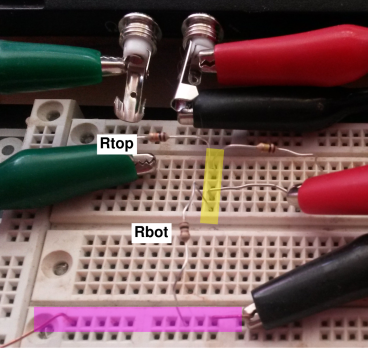 Figure 8
: Resistor Network, Presenting a Low Impedance to the Input
All the contacts in the yellow-shaded region are connected together
by the matrix board, internally. Choose Rtop to be approximately
10 kΩ and Rbot to be approximately 100 Ω. Measure
the actual resistor values with the multimeter, and record
them as lo.Rtop and lo.Rbot directives in your turbid.tbd
file.
Ignore the third resistor in the diagram.
The green clip carries the signal from the computer output. The red
clip carries the low-impedance signal from the voltage divider to
the computer input. The black clip is the ground connection. This
color-code is based on the standard color-coding of computer audio
ports: The output port is normally green, while the mic-in port is
normally pink, as in figure 9 for example.
Where the wires are coiled up, they are carefully coiled with an
even number of turns, with an equal number of clockwise and
counterclockwise turns, so that they do not act like pickup
coils.
-
We assume the input data path was configured
correctly, qualitatively, as discussed in section 4.3. Make sure your turbid.tbd file contains the
appropriate gVout, Rout, lo.Rtop and lo.Rbot directives, so that
turbid knows about the values you have already determined.
Now we want to calibrate the input impedance and gain,
quantitatively. Fire up turbid sine .01. Choose sine
amplitude that is about 10 times less than what was previously
considered normal. That’s because we expect the input to
be several hundreds of times more sensitive than the output,
and the voltage divider gives us “only” a factor of 100
attenuation.
Select the Low Z tab on the turbid gui. Verify that the Rtop and
Rbot numbers are correct. If not, correct them on the turbid gui
(for now) and in the turbid.tbd file (for next time). The Rtap
number should be zero. Leave it that way, but click on that entry
box and hit <Return>.
Every time you hit <Return>, turbid should send to standard
output an oripoint line, plus some comments.
Repeat the measurement to see whether the results are reproducible.
Change the Sine Ampl to see whether you get the same result. If
increasing the Sine Ampl causes the ordinate of the oripoint to
increase (more inverse gain, less gain) then the Sine Ampl is too
high. Also look at the Y value in the comments. It should be
around 0.1, certainly less than 1, but not insanely much smaller
than 0.1.
-
For the next step, you will need a shield box. The
high-impedance input will pick up stray electric fields. This will
almost certainly give you wrong answers unless you shield them using
a grounded backplane underneath the matrix board, and a grounded
shielding box above.
A lightweight metal cookie tin will do. If you don’t have a cookie
tin, an ordinary cooking pot will do. You can obtain even better
results using a small box covered with aluminum foil, as in
figure 10, although that’s more work than most people are
willing to do. For consistency and concision, we will call this the
“shield box”, no matter what it is made of.
You can use the following command
:; arecord -D hw:0 --disable-softvol -f S32_LE -r 48000 -V mono /dev/null
to display a VUmeter that gives a qualitative indication of what’s
going on. Without the shield, the signal is affected by all sorts of
strange things, such as how close you are sitting to the circuit.
With the shield in place, the signal should be much better behaved.
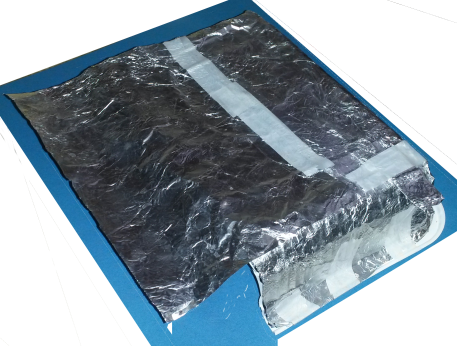 Figure 10
: Shield Box : Four Sides Covered with Aluminum Foil
Clip the grounding wire to a piece of scrap metal, so you can set it
on top of the shield box and make contact that way. That’s more
convenient than repeatedly clipping it to the box and then
unclipping.
The same logic applies underneath: If the matrix board is not already
attached to a metal backplane, find a suitable piece of metal and
bolt the matrix board to it. In an emergency, a layer of aluminum
foil suffices. Make arrangements for grounding the backplane.
-
Now we perform a measurement that is almost
the same, but presents a high impedance to the input.
Choose a value on the order of 100 kΩ for Rtap. Measure
the actual value, and add appropriate hi.Rtop, hi.Rbot, and hi.Rtap
directives in your turbid.tbd file.
Hook up the circuit shown in figure 11. It’s analogous to
the previous figure, except that now the red clip is connected to
Rtap. Cover the circuit with the shield box.
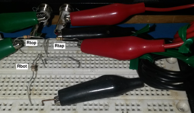 Figure 11
: Resistor Network, Presenting a High Impedance to the Input
Select the High Z tab on the turbid gui. Verify that the Rtop,
Rbot, and Rtap numbers are correct. If not, correct them on the
turbid gui (for now) and in the turbid.tbd file (for next
time). Click on the Rtap entry box and hit <Return>.
Every time you hit <Return>, turbid should send to standard output
an oripoint line, an Rin line, a bVin line, and some comments.
Repeat the measurement to see whether the results are reproducible.
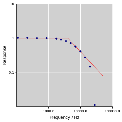
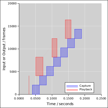
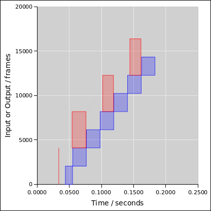
Some typical results are shown in figure 12. You can see
that turbid, when used with some skill, is capable of measuring
the input impedance to high accuracy.
lo.oripoint: 97.3, 0.001193 # lo ladder v_eff: 0.009817  r_eff: 97.3
# Y: 0.411563  lockin_mag/\muV: 490.061  sine_ampl: 0.050000

hi.oripoint: 98197.3, 0.003658 # hi ladder v_eff: 0.009817  r_eff: 98197.3
# Y: 0.134197  lockin_mag/\muV: 159.792  sine_ampl: 0.050000
# slope: 2.512340e-08  intercept: 0.001191, 0.001191
Rin: 47395.4   # ohms
bVin: 0.001191   # volts per hin

hi.oripoint: 31997.3, 0.001995 # hi ladder v_eff: 0.009817  r_eff: 31997.3
# Y: 0.246005  lockin_mag/\muV: 292.925  sine_ampl: 0.050000
# slope: 2.514615e-08  intercept: 0.001191, 0.001191
Rin: 47352.4   # ohms
bVin: 0.001191   # volts per hin

hi.oripoint: 98197.3, 0.003659 # hi ladder v_eff: 0.009817  r_eff: 98197.3
# Y: 0.536591  lockin_mag/\muV: 638.834  sine_ampl: 0.200000
# slope: 2.513894e-08  intercept: 0.001191, 0.001191
Rin: 47358.5   # ohms
bVin: 0.001191   # volts per hin
5 Background: Basic Notions
5.1 Turbid: Basic Features
Turbid is meant to be easy to use, yet robust enough to handle a wide
range of applications, including high-stakes adversarial applications.
It is a Hardware Randomness Generator (HRNG). Sometimes people call
it a True Randomness Generator (TRNG) which means the same thing. In
any case, perfect randomness is not possible.
This stands in contrast to garden-variety “Random Number Generators”
that may be good for non-demanding applications, but fail miserably if
attacked. See reference 2 for a discussion of the range of
applications, and of some of the things that can go wrong.
We now explain some theoretical ideas that will be important:
- We start with a raw input, typically the electrical noise
produced by a good-quality sound card. This noise is generated
entirely by the components on the card, in accordance with the
immutable laws of thermodynamics. It is not acoustical noise, and no
microphone is involved.
- We ascertain a reliable lower bound on the amount of
randomness in the raw input. We quantify this in terms of
adamance, as explained in reference 2. This is
calculated from basic physics principles plus a few easily-measured
macroscopic properties of the sound card. (This stands in stark
contrast to other approaches, which obtain a loose upper bound based
on statistical tests on the data.)
- We collect and concentrate the randomness. Concentration allows
us to produce an output that is random enough for all practical
purposes. This is provably correct under mild assumptions.
- We use no long-term internal secret state and therefore require
no seed.
- No noise source is perfect. Therefore we use a cryptographic
hash function to concentrate the available randomness. The
turbid motto is:
You can do more with physics and algorithms together
than you can with either one separately.
|
|
|
|
We have implemented a generator using these principles. Salient
engineering features include:
- It costs next to nothing. It uses the thermal fluctuations
intrinsic to the computer’s audio I/O system. Most computers nowadays
come with an audio chip built into the mainboard, whether you want it
or not. In the rare cases where the built-in audio system is absent,
or is needed for other purposes, a USB dongle can be used to provide
turbid with the necessary raw data, at a cost of only a few
dollars.
- It emphatically does not depend on imperfections in the
audio I/O system. Indeed, high-quality sound cards are much more
suitable than low-quality ones. It relies on fundamental physics,
plus the most basic, well-characterized properties of the audio
system: gain and bandwidth.
- It can produce thousands of bytes per second of output.
- Remarkably little CPU time is required.
- Best performance and maximally-trustworthy results depend on
proper calibration of the hardware. This needs to be done only once
for each make and model of hardware, but it really ought to be done.
Turbid provides extensive calibration features. Indeed virtually
all all of the complexity is devoted to calibration.
- The package includes optional integrity-monitoring and
tamper-resistance capabilities.
5.2 How to Define Randomness, or Not
If you ask three different people, you might get six or seven
different definitions of “random”.
At a minimum, we need to consider the following ideas:
- At one extreme there is perfect randomness.
The output is completely and unconditionally unpredictable.
- There is also pseudo-randomness, which means that there is a
pattern, but it is computationally infeasible for the adversary to
discover the pattern, so long as we keep secret the pattern and the
method we used for generating the pattern. For a wide range of
purposes, the adversary finds this to be just as unpredictable
perfect randomness.
- At the opposite extreme, there is perfect determinism, i.e.
no randomness at all, such as a source that produces an endless
string of bytes all the same, or perhaps successive digits of π,
or some other easily-recognizable pattern.
- There is also something I call squish, which is neither
reliably predictable nor reliably unpredictable. See figure 13.
For example: Once upon a time I was working on a project that
required a random generator. The pointy-haired boss directed me to
get rid of my LFSR and instead use the value of the program counter
(PC) as saved by the last interrupt, because that was
«unpredictable». I kid thee not. In fact the PC was a terrible
RNG. Successive calls tended to return the same value, and even if
you got two different values, one of them was likely to be the PC of
the null job (which was hardly surprising, since it was an
event-driven system).
I tried to explain to him that even though the PC was not
reliably predicatable, it was not reliably
unpredictable. In other words, it was squish, with no useful lower
bound on the amount of randomness.
- Combinations of the above. For example, there could be a
distribution over 32-bit words having a few bits of randomness in
each word, with the other bits being deterministic and/or squish.
Figure 13 shows a simplified view of the space of
possibilities. Note that randomness and pseudorandomness are not the
same thing, but this diagram assumes they are more-or-less equally
unpredictable, from the adversary’s point of view.
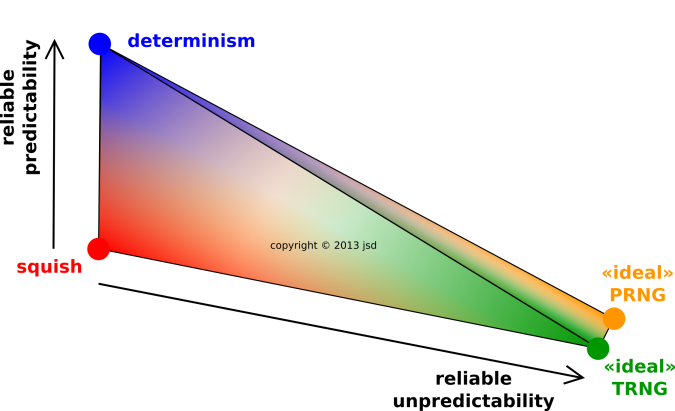 Figure 13
: Predictability, Unpredictability, and Squish
The terminology is not well settled. I have heard intelligent experts
call items 1, 2, 4, and 5 on the previous list “random”. I have
also heard them call items 3, 4, and 5 “non-random” or “not really
random”. Sometimes even item 2 is included in the catagory of “not
really random”.
We consider the terms “random” and “non-random” to be vague,
clumsy, and prone to misunderstanding. If a precise meaning is
intended, careful clarification is necessary. This remains something
of an unsolved problem, especially when talking about PRNGs.
Beware that in the cryptology community, the word «entropy» is
rather widely abused. Sometimes it is thrown around as an all-purpose
synonym for randomness, even in situations where the signal contains
absolutely no real physics entropy. This is a bummer, because in
physics, entropy has an agreed-upon, specific, and exceedingly
useful meaning.
On the other hand, in the long run it’s not much of a problem, because
it turns out that the physics entropy was almost certainly never what
you wanted anyway. There exist distributions where the entropy is
infinite but the adamance is only two bits. An adversary would have a
rather easy time guessing some outputs of such a distribution, even
though the entropy is infinite.
The essential concept here is probability distribution.
The entropy is only one property of the distribution. See
reference 2 for more discussion of this point.
In this document, and in reference 2, we use the word
“entropy” in the strictest sense: “entropy” means physics entropy.
The terms entropy and adamance are assigned very formal,
specific meanings.
- Black-versus-white extremism is unhelpful. As you can see in
figure 13, there is a large and important gray area.
- Something that is “random enough” for one application might be
not nearly random enough for another application.
5.3 TRNG versus PRNG
The contrast between a TRNG and a PRNG can be understood
as follows:
|
A Pseudo-Random Generator (PRNG) depends on an internal state
variable. That means that if I wanted to, I could give my friend a
copy of my PRNG (including the internal state) and then his PRNG
would produce the same outputs as my PRNG.
|
|
A True Random Generator
(TRNG) such as a Hardware Random Generator (HRNG) has the property
that the outputs are unpredictable in principle. It does not have
any internal state. If I give a copy to my friend, not only can he
not predict the output of my TRNG, I cannot even predict the output
of my own TRNG.
|
|
A high-quality PRNG depends on the assumption that it is
computationally infeasible for any adversary to infer the
internal state by observing the outputs. More generally, the
assumption is that the adversary will find it not worthwhile to
infer the internal state. This is a moving target, depending to
some degree on the value of whatever the pseudo-random distribution
is protecting.
|
|
A proper TRNG does not have any internal state. It
does not need to be initialized.
|
|
Every PRNG depends on some crucial assumptions, namely the
existence of a one-way function that is resistant to cryptanalytic
attack.
|
|
To a lesser extent, the same is true for every practical
HRNG that I know of.
|
|
This is probably not a serious limitation for a
well-implemented PRNG. That’s because all of modern cryptography
relies on similar assumptions. If these assumptions were to break
down, the RNG would be the least of your problems. Still, one
should always keep in mind that these assumptions are unproven.
|
|
This is even less of a problem for a HRNG, because any attack
will be much more difficult to carry out. It is a known-codetext
attack, with vastly less codetext available.
|
6 Randomness in the Raw Data
6.1 Users and Analysts
Note the contrast:
- The goal is to make using turbid as easy as possible, so that
a wide range of ordinary folks can use it without hassle. By way of
analogy, there are a lot of people who can play a piano who wouldn’t
want to build one from scratch, or even tune one.
- We also need a few specialists who know how to tune a piano.
Similarly, we need a few specialists who understand in detail how
turbid works. Security requires attention to detail. It requires
double-checking and triple-checking.
Understanding turbid requires some interdisciplinary skills. It
requires physics, analog electronics, and cryptography. If you are
weak in one of those areas, it could take you a year to catch up.
6.2 Principles versus Intution
This section exists mainly to dispel some misconceptions. Sometimes
people decide that the the laws of physics do not apply to
electronics, or decide on the basis of “intuition” that the noise in
their audio system is negligible. If you do not suffer from these
particular misconceptions, feel free to skip to section 6.3.
- For many decades, ever since the dawn of the computer age,
mathematicians and algorithm designers have tried and failed to
find an algorithm for generating randomness. There is a solution to
this problem, but the solution requires thinking outside the
“mathematical algorithm” box:
- It requires physics, especially thermodynamics and the classical
theory of fields. It is beyond the scope of this document to explain
such things. A good place to start is reference 4.
- It requires analog electrical engineering. A fine introduction
can be found in reference 5. An survey of electronic noise
processes can be found in reference 6.
- It requires conventional cryptologic algorithms such
as hash functions.
- Intuition based on digital electronics can be misleading when
extended to analog electronics.
|
A digital logic gate has considerable noise immunity. Noise,
if it is not too large, is eliminated at every step. This requires
both nonlinearity and power dissipation.
|
|
A linear analog system
cannot eliminate noise in the same way. The fundamental
equations of motion do not allow it.
|
- Humans often do not pay much attention to noise. In an ordinary
home situation, there is a considerable amount of background noise
coming from household appliances, air conditioning, the wind in the
trees outside, et cetera. In a concert hall, there is noise from
audience members fidgeting in their seats. There is also noise from
your own breathing and heartbeat. People learn to ignore these
things. It may be that you have never noticed the thermal noise that
is present in audio systems, but it is there nevertheless.
- In a typical audio system, the input impedance is considerably
greater than the output impedance. The noise level is proportional to
the resistance, as has been well observed and well explained since
1928 (reference 7 and reference 8). When line-out
is connected to line-in, the input impedance is largely shorted out
... but if the same line-in port is open-circuited, we see the full
input impedance, so there is two or three orders of magnitude more
noise than you might have expected.
- Consumer-grade microphones tend to have high impedance and/or
low signal levels. Therefore it is fairly common to find audio
systems that can apply additional analog gain to the mic-in signal,
upstream of the analog-to-digital converter. This can increase the
amount of observable noise by another two orders of magnitude.
6.3 Choice of Input Device
In principle, there are many physical devices that could be used as
the source of raw randomness. We prefer the audio system (the
“soundcard”) because such things are cheap, widely available, and
easy to calibrate. We have a provable lower bound on the rate at
which they produce randomness, and this rate in sufficient for a wide
range of applications. This provides a way to make typical hosts very
much more secure than they are now.
In contrast, a video frame-grabber card would produce randomness more
copiously, but would be much more costly. Calibration and
quality-assurance monitoring would be much more difficult.
There are many other sources that “might” produce usable randomness,
but for which a provable nonzero lower bound is not available.
6.4 Lower Bounds are Necessary
As mentioned before, we need a lower bound on the amount of randomness
per sample. This is needed to ensure that the hash function’s buffer
contains “enough” randomness, as discussed in reference 2.
Let us briefly explore the consequences of mis-estimating the
amount of randomness in the raw data:
- 1a) If we make a slight overestimate, it
means that the hash function, rather than putting out 2160
different outputs, will put out some rather smaller ensemble.
In mild cases this may not be noticeable in practice.
- 1b) A major overestimate may allow an adversary to focus
an attack on the few output-words being produced.
- 2a) If we modestly underestimate the amount of randomness
in the raw data, there is no serious harm done.
- 2b) A major underestimate will reduce the total randomness
production capability of the machine. This means the processes that
consume random symbols may block, waiting for the HRNG to produce a
usable output.
6.5 Other Contributions to the Audio Signal
We looked at the power spectrum of the signal produced by a number of
different sound cards. Based on these observations, and on general
engineering principles, we can list various hypotheses as to what
physical processes could be at work, namely:
- Johnson noise, due to thermal fluctuations in the front-end
input resistor.
- Johnson noise in other resistors and dissipative elements
later in the processing chain.
- Shot noise and generation/recombination noise, arising in
small structures because electrons are not infinitely small.
- 1/f noise.
- Hum at powerline frequency and harmonics thereof.
- Interference from other subsystems such as video cards and
switching power supplies.
- Sums of the above.
- Intermodulation. For example, intermodulation occurs when we
digitize a superposition of fairly-low-amplitude hum plus
very-low-amplitude high-frequency noise. That’s because the digitizer
is sensitive to the high-frequency noise component only when the hum
component is near one of the digitizer steps.
- Various filter functions applied to the above.
- Deceptive signals injected by an adversary.
Some of these are undoubtedly fine sources of randomness. The only
problem is that except for item #1, we cannot calculate their
magnitude without a great deal more engineering knowledge about the
innards of the card. Using these sources might produce a HRNG that is
correct, but not provably correct. Since we want something that is
provably correct, we simply ignore these other contributions. They
can’t hurt, and almost certainly provide a huge margin of safety.
That is: We need randomness in the raw data, and we need to
know a provable lower bound on the amount of randomness. Turbid
consistently applies the principle that having extra randomness
is OK, and underestimating the amount of randomness is OK.
This may give us less-than-optimally efficient use of the available
randomness, but it guarantees correctness. Turbid consistently
chooses correctness over efficiency.
6.6 Examples of Soundcard Properties
Just to help you get the lay of the land, here are the key
characteristics of a few soundcards. The older cards are of
historical interest only. More recent cards perform better.
| Card | Q / µV
| RIn / Ω
| Kout
| B
| N
| σ / µV
| s / bits
| ROut / Ω |
| Deskpro onboard | 6.6 | 8800 | .154 | 18500 | 48000 | 1.63 | 0.3 | |
| Delta-1010 (pro) | 0.22 | 3020 | .223 | 36500 | 96000 | 1.28 | 4.65 | 192 |
| Delta-1010 (con) | 1.31 | 11000 | 1.24 | 36500 | 96000 | 2.55 | 3.04 | 1005 |
| Thinkpad
cs4239 (Line) | 19.6 | 7900 | .037 | 9000 | 44100 | 1.07 | 0 | |
| Thinkpad
cs4239 (Mike) | 1.65 | 10100 | .038 | 7300 | 44100 | 1.09 | 1.58 | |
| Extigy (Line) | 22.5 | 20200 | .327 | 18000 | 48000 | 2.4 | 7e-5 | |
| Extigy (Mike) | 12.4 | 6100 | .332 | 12000 | 48000 | 1.1 | 3e-7 | |
Note that the CT4700 reports itself as “ENS1370” so it uses the ens1370.ctl
control file.
7 The Role of Measurement and Testing
7.1 Issues of Principle; Cat and Mouse
By way of analogy, let us consider the relationship between
code-breakers and code-makers. This is a complex ever-changing
contest. The code-breakers make progress now and then, but the
code-makers make progress, too. It is like an “arms race” but much
less symmetric, so we prefer the term cat-and-mouse game.
At present, by all accounts, cryptographers enjoy a very lopsided
advantage in this game.
There is an analogous relationship between those who make PRNGs
and those who offer tools to test for randomness. The PRNG has
a hidden pattern. Supposedly the tester “wants” the
pattern to be found, while the PRNG-maker doesn’t.
We remark that in addition to the various programs that bill
themselves as randomness-testers, any off-the-shelf compression
routine can be used as a test: If the data is compressible, it
isn’t random.
To deepen our understanding of the testing issue, let’s consider the
following scenario: Suppose I establish a web server that puts out
pseudo-random bytes. The underlying PRNG is very simple, namely a
counter strongly encrypted with a key of my choosing. Each weekend, I
choose a new key and reveal the old key.
The funny thing about this scenario is the difference between last
week’s PRNG and this week’s PRNG. Specifically: this week’s PRNG will
pass any empirical tests for randomness that my adversary cares to
run, while last week’s PRNG can easily be shown to be highly
non-random, by means of a simple test involving the now-known key.
As a modification of the previous scenario, suppose that each weekend
I release a set of one billion keys, such that the key to last week’s
PRNG is somewhere in that set. In this scenario, last week’s PRNG can
still be shown to be highly non-random, but the test will be very
laborious, involving on the order of a billion decryptions.
Note that to be effective against this PRNG, the randomness-testing
program will need to release a new version each week. Each version
will need to contain the billions of keys needed for checking whether
my PRNG-server is “random” or not. This makes a mockery of the idea
that there could ever be an all-purpose randomness tester. Even a
tester that claims to be “universal” cannot be universal in any
practical sense.2 An all-purpose randomness tester would be
tantamount to an automatic all-purpose encryption-breaking machine.
7.2 Necessary but Not Sufficient
To paraphrase Dijkstra: Measurement can prove the absence of
randomness, but it cannot prove the presence of randomness. More
specifically, any attempt to apply statistical tests to the output of
the RNG will give an upper bound on the amount of randomness, but what
we need is a lower bound, which is something else entirely.
As described in reference 2, we can calculate the amount of
randomness in a physica process, based on a few macroscopic physical
properties of the hardware. It is entirely appropriate to measure
these macroscopic properties, and to remeasure them occasionally to
verify that the hardware hasn’t failed. This provides a lower bound
on the randomness, which is vastly more valuable than a
statistically-measured upper bound.
As discussed in reference 2, tests such as Diehard
(reference 9) and Maurer’s Universal Statistical Test
(reference 10) are far from sufficient to prove the correctess of
turbid. They provide upper bounds, whereas we need a lower bound.
When applied to the raw data (at the input to the hash function) such
tests report nothing more than the obvious fact that the raw data is
not 100% random. When applied to the output of the hash function,
they are unable to find patterns, even when the density of randomness
is 0%, a far cry from the standard (100%) we have set for ourselves.
A related point: Suppose you suspect a hitherto-undetected weakness in
turbid. There are only a few possibilities:
- If you think there is a problem with SHA-1, it would make more
sense to attack SHA-1 by conventional means, including artfully chosen
inputs, as opposed to haphazardly probing it with whatever raw data is
coming off the data-acquisition system.
- If you think the problem is upstream of SHA-1, you should
instrument the code and look there, at the input to SHA-1.
Running the allegedly problematic data through SHA-1 and looking
at the output is like looking through the wrong end of a really long
telescope; it greatly reduces your ability to see anything of
interest.
- Probably the best chance of getting a non-null result from a
“randomness test” is if there is a gross bug in the control logic,
such as forgetting to write the result to the output. For this to
work, you need to turn off (or bypass) the error concealment as
discussed in section 8.
The foregoing is a special case of a more general rule: it is hard to
discover a pattern unless you have a pretty good idea what you’re
looking for. Anything that could automatically discover general
patterns would be a universal automatic code-breaker, and there is no
reason to believe such a thing will exist anytime soon.
There are some tests that make sense. For instance:
- The program checks the supposed LSB (Least Significant Bit) of
the raw data to make sure it is in fact significant – not stuck or
easily predictable from the higher bits.
- If you don’t believe the theoretical arguments, you could test
the theory by (temporarily!) substituting a crippled hash function
(producing, say, 8-bit hashcodes rather than 160-bit hashcodes). Then
the statistical tests might have a chance of detecting problems
upstream of the hash function, e.g. a miscalculation of the density of
randomness in the raw data.
On the one hand, there is nothing wrong with making measurements, if
you know what you’re doing. On the other hand, people have gotten
into trouble, again and again, by measuring an upper bound on the
randomness and mistaking it for a lower bound.
The raison d’etre of turbid is that it provides a reliable
lower bound on the density of randomness, relying on physics, not
relying on empirical upper bounds.
7.3 Actual Measurement Results
We ran Maurer’s Universal Statistical Test (reference 10) a few
times on the output of turbid. We also ran Diehard. No problems
were detected. This is totally unsurprising, and it must be
emphasized that we are not touting this a serious selling point for
turbid; we hold turbid to an incomparably higher standard. As
discussed in section 7.2, for a RNG to be considered
high quality, we consider it necessary but nowhere near sufficient for
it to pass statistical tests.
7.4 Summary
To summarize this subsection: At runtime, turbid makes specific
checks for common failures. As discussed in section 7.3 occasionally but not routinely apply
general-purpose tests to the output.
We believe non-specific tests are very unlikely to detect deficiencies
in the raw data (except the grossest of deficiencies), because the
hash function conceals a multitude of sins. You, the user, are
welcome to apply whatever additional tests you like; who knows, you
might catch an error.
8 Error Detection versus Error Concealment
8.1 Basics
We must consider the possibility that something might go wrong with
our randomness generator. For example, the front-end transistor in
the sound card might get damaged, losing its gain (partially or
completely). Or there could be a hardware or software bug in the
computer that performs that hashing and control functions. We start
by considering the case where the failure is detected. (The
other case is considered in section 8.2.)
At this point, there are two major options:
- Throtting: We can make the appropriate (partial or
complete) reduction the rate at which turbid emits symbols, so that
whatever symbols are emitted continue to have the advertised high
density of randomness.
- Concealment: We can conceal the error and continue to emit
symbols at the same old rate. This means that turbid has been
degraded from a high-quality randomness generator to some kind of
PRNG.
We can ornament either of those options by printing an error message
somewhere, but experience indicates that such error messages tend
to be ignored.
If the throttling option is selected, you might want to have
multiple independent generators, so that if one is down,
you can rely on the other(s).
The choice of throttling versus concealment depends on the
application. There are plenty of high-grade applications where
concealment would not be appropriate, since it is tantamount to
hoping that your adversary won’t notice the degradation of your
random generator.
In any case, there needs to be an option for turning off – or
bypassing – error concealment, since it interferes with measurement
and testing as described in section 7.
8.2 Combining Generators
We can also try to defend against undetected flaws in the
system. Someone could make a cryptanalytic breakthrough, revealing a
flaw in the hash algorithm. Or there could be a hardware failure that
is undetected by our quality-assurance system.
One option would be to build two independent instances of the
generator (using different hardware and different hash algorithms) and
combine the outputs. The combining function could be yet another
hash function, or something simple like XOR.
9 Context, History and Acknowledgments
For a discussion of the Fortuna class of random generators, and
how that contrasts with turbid, see reference 11.
For a discussion of the Linux device driver for /dev/random and
/dev/urandom, see reference 12.
There is a vast literature on hash functions in general. Reference 13 is a starting point. Reference 14 is a useful literature
survey. Reference 15 was an influential early program for
harvesting randomness from the audio system; it differs from turbid in
not having calibration features. Reference 16 uses the
physics of a spinning disk as a source of randomness.
Methods for removing bias from a coin-toss go back to von Neuman; see
reference 17 and references therein; also reference 18.
Reference 19 suggests hashing 308 bits (biased 99% toward
zero) and taking the low-order 5 bits of the hash to produce an
unbiased result. This is correct as far as it goes, but it is
inefficient, wasting 80% of the input adamance. Presumably that
reflects an incomplete understanding of the hash-saturation principle,
in particular the homogeneity property discussed in reference 2, which would have led immediately to consideration of
wider hashcodes. There is also no attempt to quantify how closely the
results come to being unbiased.
Thanks to Steve Bellovin, Paul Honig, and David Wagner for
encouragement, incisive questions, and valuable suggestions.
10 Conclusions
Practical sources of randomness can be characterized in terms of the
adamance density. The raw sources have an adamance density greater than
zero and less than 100%. The methods disclosed here make it possible
to produce an output that approaches 100% adamance density as closely
as you wish, producing symbols that are random enough for any
practical purpose. It is important to have a calculated lower
bound on the adamance density. In contrast, statistical tests provide
only an upper bound, which is not what we need.
It is possible to generate industrial-strength randomness at very low
cost, for example by distilling the randomness that is present in
ordinary audio interfaces.
A The Definition of Randomness and Surprisal
A.1 Introduction and Intuitive Examples
In order to refine our notions of what is random and what is not,
consider the following million-character strings. We start with
-
Example E1
- : “xxxxxxxx...xx” (a million copies of “x”)
That seems distinctly non-random, very predictable, not very complex.
Next, consider the string
-
Example E2
- : “xyxyxyxy...xy” (half a million copies of “xy”)
That seems also non-random, very predictable, not very complex.
-
Example E3
- : “31415926...99” (the first million decimal
digits of π/10)
That is somewhat more interesting. The digits pass all known tests
for randomness with one narrow exception (namely tests that check for
digits of π). However, they must still be considered completely
predictable. Finally, consider the two strings
-
Example E4
- : “AukA1sVA...A5”
-
Example E5
- : “Aukq1sVN...G5”
The million-character string represented by example E5 is, as far as
anybody knows, completely random and unpredictable. Example E4 is very
similar, except that the letter “A” appears more often than it would
by chance. This string is mostly unpredictable, but contains a
small element of nonrandomness and predictability.
A.2 Definitions
Following Solomonoff (reference 20 and
reference 21) and Chaitin (reference 22) we
quantify the surprisal of a string of symbols as follows:
Let z be a string of symbols. The elements of z are denoted zk
and are drawn from some alphabet Z. The number of symbols in the
alphabet is denoted #Z.
Let PC(z) be the probability that computer programs, when run on a
given computer C, will print z and then halt. The surprisal is
defined to be the negative logarithm of this probability, denoted
$C(z) := − logPC(z). In this paper we choose to use base-2
logarithms, so that surprisal is measured in bits. Surprisal is also
known as the surprise value or equivalently the
unexpectedness. It is intimately related to entropy, as
discussed below.
Note that we are using one probability distribution (the probability
of choosing a computer program) to derive another (the
probability PC(z) of a symbol string). To get this process
started, we need to specify a method for choosing the
programs. Better yet, using the notions of measure theory, we realize
that probability need not involve choosing at all; instead all we
really need is a method for assigning weight (i.e. measure) to each of
the possible programs. Here is a simple method:3 Consider all possible programs of length
exactly L* (measured in bits, since we are representing all
programs as bit-strings). Assign each such program equal measure,
namely 2−L*. Then test each one and count how many of them
produce the desired output string z and then halt, when run on the
given computer C. The measure of a string is the total measure of
the set of programs that produce it. A string that can be produced by
many different programs accumulates a large probability.
In this construction, a short program X (i.e. one which has a length
L(X) less than L*) is not represented directly, but instead is
represented by its children, i.e. programs formed from X by padding
it with comments to reach the required length L*. There are at
least 2L*−L(X) ways of doing the padding, and each way
contributes 2−L* to the total measure. This means that a string
z that can be produced by a short programs X will have a
probability at least 2−L(X), no matter how large L* is. We
take the limit as L* becomes very large and use this in the
definition of PC(z).
Usually the probability PC(z) is dominated by (the children of) the
shortest program that produces z. Therefore some people like to use
the length of this shortest program as an estimate of the surprisal.
This is often a good estimate, but it should not be taken as the
definition.
The explicit dependence of PC(z) on the choice of computer C
calls attention to an element of arbitrariness that is inherent in any
definition of surprisal. Different people will assign different
values to “the” surprisal, depending on what resources they
have, and on what a priori information they have about the
situation.
In an adversarial situation such as cryptography, we suggest that
probabilities be defined in terms of the adversary’s computer.
If you have multiple adversaries, they can be treated as a single
adversary with a parallel computer.
A.3 Properties of the Surprisal
In this section, for conciseness, we drop the subscript C ... but
you should remember that the probabilities and related quantities are
still implicitly dependent on the choice of C.
-
- Upper bound: If z is a string of bits, the surprisal
$(z) can never exceed the length L(z) by more than a small
amount, because we can write a program that contains z and just
prints it verbatim. More generally, if z is a string of symbols,
$(z) can never exceed L(z) log(#Z) by more than a
small amount. Again, that’s because we can write a program that
contains a literal representation of z and just prints it verbatim.
- Tighter Upper Bound: The surprisal cannot exceed the
length of the compressed representation4 of z by more than a
bounded amount, because we can write a program that contains the
compressed representation and calls the uncompress utility.
- Lower Bound: With very few exceptions, the surprisal $(z) of
any string z cannot be not much less than L(z) log(#Z). You can
see why this must be so, using a simple pigeon-hole argument: Consider
all bit-strings of length 500, and suppose that a certain subset
contains 1% of the strings but still has 490 bits of entropy. Well,
then we are talking about 1% of 2500 strings, each having
probability 2−490 — which adds up to more than 100%
probability. Oops.
A.4 Limitations
A relatively minor objection to this definition of surprisal is
that PC(z) includes contributions from arbitrarily-long programs.
That is a problem in theory, but in practice the sum is dominated by
relatively short programs, and the limit converges quickly.
A much more serious objection is that even for modest-sized programs,
the definition runs afoul of the halting problem. That is, there may
well be programs that run for a million years without halting, and we
don’t know whether they would eventually produce string z and
then halt. This means the surprisal, as defined here, is a
formally uncomputable quantity.
We will duck both these issues, except for the following remarks.
- Any compressed representation that you happen to find for z
puts a lower bound on PC(z) and an upper bound on the surprisal
$(z).
- There do exist compression algorithms that are computable
(indeed efficiently computable) and are effective on certain types of
signal. These algorithms, as a rule, make use of specialized
knowledge about the type of signal (text, voice, music, video, et
cetera).
A.5 Surprise Density
In this section we shift attention from the unpredictability of
strings to the unpredictability of the individual symbols making up
the string.
Let us re-examine the examples given at the beginning of this section.
Example E5 has surprisal $(z) very close to L(z) log(#Z).
We classify strings of this sort as absolutely-random, by which
we mean algorithmically-random.
Examples E1, E2, and E3 all have surprisal much less than their
length. These strings are clearly not absolutely-random.
The interesting case is example E4. Intuitively, we think of this as
“somewhat unpredictable” but more predictable than E5. To make this
notion quantitative, we introduce the notion of surprise
density. The following quantity tells us the surprise density of the
string z in the region from i to j:
|
σj|i(z) := | | $(Front(z, j)) − $(Front(z,i)) |
|
| j−i |
|
(1) |
where Front(z,i) is the substring formed by taking the first i
symbols of the string z.
The surprise density for examples E1, E2, and E3 is zero for any region
not too near the beginning. The surprise density for example E5 is as
large as it possibly could be, namely 100% of log(#Z). Example
E4 illustrates the interesting case where the surprise density is quite
a bit greater than zero, but not quite 100% of log(#Z).
As mentioned in section 5.2, we consider the unadorned term
“random” to be ambiguous, because it means different things to
different people. Some people think “random” should denote 100%
surprise density, and anything less than that is “non-random” even
if it contains a great deal of unpredictability. Other folks think
that “random” refers to anything with an surprisal density greater
than zero, and “non-random” means completely predictable. Yet other
folks extend “random” to include pseudo-random strings, as long as
they are “random enough” for some application of interest. Even
some professionals in the field use the word this way; reference 23 and the more recent
reference 24
speak of “deterministic random number generators”,
although it could be argued that it is impossible in principle for a
process to be both deterministic and random. The randomness of a PRNG
comes from the seed. Calling a PRNG “deterministic” seriously
understates the importance of the seed.
In the space of all possible strings, almost all strings are
absolutely-random, i.e. are algorithmically-random, i.e. contain 100%
surprise density. However, the strings we find in nature, and the
strings we can easily describe, all have very little surprise density.
We can summarize this by saying: “All strings are absolutely-random,
except for the ones we know about”.
We can use similar ideas to describe PRNGs and contrast them with
HRNGs.
|
Most of modern cryptography revolves around notions of
computational intractability. (I’m not saying that’s good or bad; it
is what it is.
|
|
In contrast, there is another set of notions,
including adamance, entropy, and the related notion of unicity
distance, that have got nothing to do with computational
intractability.
|
|
The long strings produced by a good PRNG are conditionally
compressible in the sense that we know there exists a shorter
representation, but at the same time we believe them to be
conditionally incompressible in the sense that the adversary has no
feasible way of finding a shorter representation.
|
|
The long strings
produced by a HRNG are unconditionally, absolutely incompressible.
Specifically, the set of strings collectively cannot be compressed at
all. As for each string individually, it is not compressible either,
except possibly for trivially rare cases and/or trivial amounts of
compression.
|
B Soundcard Quirks
B.1 General Observations
This section is a collection of details about certain soundcards.
(You can refer back to table 2 for a summary of the
performance of a few soundcards. Also, section 4 provides
step-by-step procedures that apply to “generic” soundcards.)
Soundcards generally include mixer functions. You have to initialize
the mixer, to set the sliders on the features you want and/or to set
the switches to bypass the features you don’t want. This is a bit of
a black art, because the soundcards typically don’t come with any
“principles of operation” documentation.
Graphical user interface (GUI) programs such as alsamixer may
help you make some settings, but may not suffice to fully configure
the mixer. All too often, the card has “routing switches” and other
features that the GUI doesn’t know about. A reasonable procedure that
gives complete control is to invoke “alsactl -f record.ctl
store”, edit record.ctl, then “alsactl -f record.ctl restore”.
Or you can use amixer to fiddle one setting without disturbing others.
B.2 Intel High-Definition Audio
The Intel High-Definition Audio spec (reference 25) describes the
codec but says remarkably little about mixer functions.
B.3 Extigy
This is yet another example of hype and deception from Creative Labs.
The device itself, the box it comes in, and the advertising all
prominently mention USB, 24-bit audio, and 96 kHz sampling rates.
However, according to all available evidence, the device will not
transmit 24-bit audio via USB to the DACs or from the ADCs (no matter
what the data rate). It also will not transmit 96 kHz samples via USB
to the DACs or from the ADCs (no matter what the word size).
Apparently the only way in which the Extigy can deal with 24 bits or
96 kHz is by shipping it digitally (e.g. via S/PDIF) to/from some
other device.
It also has astonishingly poor input sensitivity. It’s about 5 times
worse than a typical cheap sound card, and about 100 times worse than
a decent 24-bit soundcard, as you can see from table 2.
The Extigy is no good for present purposes. I recommend you do not
buy this product. Many other Creative Labs products have problems,
too, so in fact I recommend that you never buy anything made by them.
B.4 M-Audio Delta 1010
This is a high-end system, with eight analog inputs, eight analog
outputs, 96000 frames per second, and 24 bits of resolution. M-Audio
was previously known as Midiman.
Each of the eight analog input and each of the eight analog outputs
has a pushbutton that I call the “pro/con” switch.
Professional studio equipment (pro) runs at lower impedances and lower
signal levels than consumer-grade home audio equipment (con). That
is, the pro setting (switch pushed in) means lower impedance and lower
open-circuit voltage on output, and lower impedance and greater
voltage-sensitivity on input. Whether you care about the lower
impedance depends on the impedance of whatever the card is hooked to.
The card does not have an 8×8 or 10×10 mixer board.
It is apparently 10×2. We bypass it, as discussed below.
The alsa driver always expects 10 channels of output: 8 analog plus 2
S/PDIF. If you are only interested in a subset thereof, you have to
pad things so the buffer has 10 samples per frame anyway. Similarly,
the alsa driver always produces 12 samples per frame on input: 8
analog plus 2 S/PDIF plus 2 from the mixer. For present purposes we
use the 8 analog inputs and ignore the others, since they contain
no additional randomness. Therefore you must pass the
--channel-mask 255 option to turbid; otherwise the
program will have less randomness than it thinks it has,
by a factor of 8/12ths.
Each of the eight analog inputs is always routed directly to its own
DAC, so the PCM input functionality is always unaffected by the sliders
and switches on the mixer.
The routing can be set so that each of the eight analog outputs is fed
directly from the PCM data. This is recommended. This makes the PCM
output functionality independent of the sliders on the mixer.
B.5 Thinkpad 600
Getting this to work requires the following tricks:
- Make sure “quick boot” is turned off. (If it is turned on,
it tells the BIOS to skip configuration of PnP devices – not good.)
Press and hold F1 during boot-up to get to the BIOS setup.
- After you’ve done that, run IBM’s DOS-mode Thinkpad utilities
to enable the sound system and find out what resources it is using
(registers, IRQs, and DMA channels). It is (just barely) possible to
make a bootable 1.44MB floppy containing the DOS operating system plus
the IBM utilities. The utilities come from IBM as a self-extracting
executable, which you will have to unpack on a Windows machine and
then move to the floppy.
- Beware that the ALSA drivers may have a reversed notion of
what is DMA0 and what is DMA1. If it almost works, try reversing
their settings in /etc/modules.conf.
As usual, you will need the .ctl file (included in the turbid
bundle) plus the settings in table 2.
The same jack doubles as a Line-In port and Mike-In port, depending on
software settings. Unlike the typical Mike-In port as described in
section 4.3, this Mike-In port is stereo and does
not provide power to the microphone. This would be bad if you wanted
to connect a microphone that needed power, but it’s ideal for our
purposes. Basically it’s like an ordinary Line-In port, with higher
sensitivity.
C Bandwidth Measurement
For reasons discussed in reference 8, the Johnson noise in
any Ohmic resistor is nice white noise. Voltage samples are
independent and identically distributed (IID), according to a Gaussian
normal distribution with zero mean and variance given by
where k is Boltzmann’s constant, T is the temperature (300 K), B
is the bandwidth, and the brackets ⟨⋯⟩ denote the
ensemble average.
The bandwidth is essentially the average of gain squared, averaged
over all frequencies. We care about the square of the gain, because
in equation 2 we care about the square of the
voltage.
The principle of the bandwidth measurement is as follows: Equation 2 tells us the variance of the voltage right at the
resistor. The quantity we actually measure has been amplified,
according to some gain function G which depends on frequency. So a
more complete description is
|
σo2 = | ∫ | | 4 k T R |G(f)|2 df
(3) |
where the subscript o on σo indicates this is the quantity
we observe, and fmax is some “large enough” frequency; the
real, relevant bandwidth B is hidden in G, which goes to zero at
large frequencies. Since G is presumably an even function of
frequency, we can rewrite this as
|
σo2 = | ∫ | | 2 k T R |G(f)|2 df
(4) |
and in a discrete (sampled) system this becomes
|
σo2 = | | 2 k T R |G(k Δf)|2 Δf
(5) |
where we identify the sampling frequency N = MΔf = 2 fmax,
covering the whole range of positive and negative frequencies. We can
write this in the suggestive form
where G*2 is some nominal mid-band power gain, if we identify
and we call B the power-averaged bandwidth.
By definition the gain G is Vo / Vr, where Vr is the
voltage right at the resistor, and Vo is what we observe.
This expression applies to any Vo/Vr ratio, whether Vr comes
from thermal noise or from any other source.
We choose to inject a non-thermal probe signal Vr. It is
constructed to be “white” – i.e. it has constant magnitude
independent of frequency. That allows us to pull it outside the
summation:
and by Parseval’s theorem we can rewrite that frequency-domain
expression as a time-domain expression
It is easy to get a good lower bound on B. At compile time, we know
the root-mean-square (RMS) magnitude of the internal representation of
the probe signal; by construction it is -15dBFS. Then given K and
R (and Zref) we know ⟨Vr2⟩ in the
passband. At frequencies outside the passband this voltage will roll
off a little, because of the anti-aliasing filter in the soundcard
output stage. This will cause us to under-estimate B by a little,
which is harmless. Finally we determine ⟨Vo2⟩ by
summing the squares of the observed voltage samples and multiplying by
the appropriate calibration factors (involving Q).
You might have thought based on the form of equation 3 that we
would need to take a Fourier transform, but we don’t, because of
Parseval’s theorem.
D Units: Hin, Bath and dBh
In the turbid software, whenever possible, calculations use SI
units, so that when a voltage variable takes on the floating-point
value 1.0, that means one SI volt.
However, that is not always possible. For example, raw input signals
as they come from the hardware, before calibration, are represented as
integers. We can renormalize such integers as fixed-point fractions,
as a fraction of full scale. We say that a full-scale deflection
corresponds to a square wave with an amplitude of 1 bath.
Similar words apply to output signals.
However, until the calibration process is complete, we don’t know the
connection between 1 bath and 1 volt.
We measure the amplitude of waves in terms of RMS amplitude. This
differs from the convention you learned in high school, which used the
peak amplitude. Therefore a 1-volt sine wave peaks at 1.4
volts. (For a square wave, the peak voltage and the RMS voltage are
the same.) Note that virtually every voltmeter on earth measures RMS
voltage. One type of meter measure the true RMS voltage, while
another type measures the peak voltage and divides by 1.4. You can
see the difference between the two types if you apply the meter to a
square wave of known amplitude. The “true RMS” meter will get the
right answer, whereas the other will give a reading that is
systematically too low.
Meanwhile, anything that is measured in dBx is measured relative to a
reference level that is 15 dB below full scale. This means that a
rail-to-rail square wave (such as might result from extreme clipping)
peaks at 1.0 ibu, has an RMS of 1.0 ibu, and a power level of +15
dBx. Similarly a sine wave that peaks at exactly 1.0 ibu has an RMS
of 0.707 ibu, and a power level of +12 dBx.
As always, a dB is a power measurement. This includes dBx. It does
not depend directly on the peak voltage. As a corollary, the peak
voltage of a zero-dBx sine wave √2 higher than the top of a
zero-dBx square wave.
E Calculating Impedances
E.1 Output
Suppose the computer’s audio output circuit has some gain g and some
Thévenin equivalent series resistance Rout, both of which we
want to determine. We connect some external load resistance and
measure the voltage. Then we connect some different load, and measure
the voltage again. If one of the loads has infinite resistance, that
gives us a direct measure of the open-circuit voltage.
During this process, the turbid output is represented in the output
buffer by a sine wave of amplitude X (RMS), measured in hins.
Therefore the open-circuit voltage is Voc = gX, which defines
what we mean by g.
On the ith measurement, the voltage observed on the meter is:
hence
So if we plot the inverse voltage gain (X/Vm, i) as a function
of the inverse resistance (1/Rload, i), we should get a
straight line with slope Rout/g and intercept 1/g.
In the turbid code, we speak of oropoints. Each oropoint is an
ordered pair, (1/Rload, X/Vm). The gain g is represented in
turbid by the variable gVout, which has dimensions of hins
per volt.
Now let’s feed the computer’s audio output circuit into an external
resistor network. The combination forms a linear circuit with some
effective Thévenin equivalent open-circuit voltage Veff and
effective series resistance Reff, both of which we can calculate
from the known properties of the circuit. These properties include
the computer’s output impedance, Rout, which is considered known,
since it was determined in section E.1. Similarly the
driving voltage Voc = gX is known, since we control X and we
calibrated g in section E.1.
We connect the output of this network to the audio input. The input
port has some input impedance Rin and some gain b, both of
which we need to determine. We can observe the digitized input signal
Yj as it appears in the input buffer, measured in hins.
hence
So if we plot the observed inverse gain Veff/Yj as a function of
the calibration network equivalent resistance Reff, j, we
should get a straight line with slope b/Rin and intercept b.
You can easily check this formula in the limiting cases Reff = 0
and Reff → ∞.
In the turbid code, we speak of oripoints. Each oripoint is an
ordered pair (Reff, Veff/Y). The inverse gain b is
represented by the variable bVin, and has units of volts per
hin.
F Noise in Voltage Dividers
For some perspectives on Johnson noise and the Nyquist formula,
including what happens when there is a frequency-dependent gain, see
reference 26.
This has some interesting implications and ramifications for our
randomness generator. There are a couple of regimes to consider:
- Suppose you have a sound card where the input impedance consists
of a nice small capacitance (high Z) and a not-so-nice smallish
resistance (low Z), such that the corner frequency 1/(2πRC) is
high compared to your digitizer’s usable bandwidth. In this regime
you don’t care about the capacitance value; the impedance of the input
is real (i.e. non-reactive) across the relevant part of the spectrum.
The amount of noise on the input is determined by the resistance. The
noise is not large (because the resistance is small), but at least
it’s nice and white, i.e. independent of frequency.
In this regime, assuming the goal is to collect noise samples, you
don’t want to add any additional resistance in parallel with what’s
already there. That would just move the flat part of the curve to a
lower voltage. (It would also push the corner frequency out to a
higher frequency, but that doesn’t do any good if the digitizer
doesn’t go that high.)
- In contrast, now suppose you have a sound card where the input
impedance consists of a significant capacitance (low Z) and a
relatively high resistance (high Z), such that corner frequency is
low compared to your digitizer’s usable bandwidth. (I’ve seen
examples of this.) The impedance is reactive across a big part of the
relevant spectrum. This is tricky, because the noise is not white.
It is pink. Successive samples of the voltage will be somewhat
correlated.
There are various ways of dealing with this.
- One possibility is to decorrelate the signal by postprocessing
it. You could do a deconvolution using Fourier methods, or you could
build a digital filter that implements the inverse of the RC filter.
- Another possibility is to accept the signal as-is, and use its
conditional randomness as our source of randomness. That is,
recognize that each sample has some conditional probability
distribution – conditioned on all of history – and as long as that
distribution has enough spread, we can use it.
In this regime it makes sense to add some resistance. This whitens
the noise. It lowers the peak noise per unit bandwidth. However,
remember that the area under the curve is independent of the
resistance. So as long as the corner frequency is not large compared
to what your digitizer can handle, you’re not losing anything by
lowering the resistance.
If the added external resistance dominates the internal resistance,
that provides a nice convenience: It means you know what the
resistance value is. This simplifies the calibration.
G ALSA Timing
Three concepts:
- The ALSA period is the interval between interrupts. The
driver catches interrupts from the hardware. For example, for the
capture direction, the driver has no idea that data is available
until the interrupt arrives. Reference: http://alsa.opensrc.org/Period
- Turbid defines an iblock and an oblock. These refer to the
amount of stuff transferred between the userland program and the
driver. Normally such things are called i/o buffers, but I call them
blocks, to avoid confusion with the following item.
The block size can plausibly be as small as the period, and as large
as the buffer. On input, a small block size seems to have little or
no effect on efficiency. In contrast, output block size seems to
have a significant effect on efficiency. Larger blocks are more
efficient. I have no clue how to explain the contrast.
- The ALSA buffer is internal to the driver. It is
typically a few times larger than the ALSA period. The buffer allows
the capture hardware to get a bit ahead of the userland program,
without causing an overrun. In the other direction, the buffer
allows the playback program to get a somewhat ahead of the game, if
it can.
G.1 Unlinked
Some observations:
- I’ve got it set up so that FrAppBuf is less than the ALSA
buffer size.
- I’ve got it set up so that appbuf__fr is greater than the
period. It makes no sense at all.
- The first readi blocks for .02 seconds. At this point the state
transitions from 2 (prepared) to 3 (running).
- The first writei does not block at all. At this point the state
transitions from 2 (prepared) to 3 (running).
Some ALSA timing is shown in figure 14. This is
peculiar in a couple of ways. For one thing, the capture i/o buffer
is a different size from the playback i/o buffer. Also, the first
readi has been artificially delayed by 10 milliseconds relative to the
first writei, just to clarify the relationship between the two
streams.
Each rectangle represents an i/o call. The bottom of the rectangle is
the number of frames (input or output) before the call, and the top is
the number of frames (input or output) after the call. Similarly the
left edge is the time at the start of the call, and the right edge is
the time upon return from the call.
In figure 14 the command was turbid show timing comb
0 freq 1000 ochan 0. You can see that the playback process has a lot
of work to do, so the corner of one red rectangle does not meet the
corner of the next. In contrast, the capture process has very little
work to do, so the rectangles very nearly meet corner-to-corner.
G.2 Linked
Now consider what happens when we use snd_pcm_link(...) to
synchronize the two streams. At the time of the first write to the
playback device, the playback stream starts running (obviously)
... and the capture stream also starts running (because it is linked).
The artificial 10 ms delay is still there, but it affects only the
left edge of the first rectangle, not the right edge.
H ALSA Hacking
Figure 16 comes from reference 27. As you can
see, the audio circuitry «supposed» to be independent of the
plug-sense circuits. However, the observed fact is that not all
computer manufacturers play by these rules. There are machines from
reputable companies where the Mic-In audio signal gets shorted to
ground when the jack is removed.
The elegant behavior suggested by figure 16 stands in
contrast to the old but not venerable AC’97 standard, as shown in
figure 17. It called for grounding the audio signals when
the plug was removed. However, 1997 was a lot of dog years ago. In
an HD Audio system, grounding is nonstandard. From the turbid
point of view, it is undesirable. It means you have to physically
plug something into the jack in order to harvest high-quality noise.
Reconfig requires that the sound card not be in use. That means you
have to shut down all of the following processes:
-
turbid
- alsamixer
- sox or arecord (which you might be using as a VU meter)
You might need to shut down some others also:
-
pulseaudio
- timidity daemon
To find who’s using the audio system, you might use the command
:; lsof | grep /dev/snd
H.1 Unloading/Reloading the Driver
To exercise the early-patch features, such as hints, you do
not need to unload the entire sound-driver stack. Unloading
and reloading the snd_hda_intel is sufficient.
        :; modprobe -r snd_hda_intel
        :; modprobe -a snd_hda_intel
H.2 Configuring the Firmware
The “early patch” firmware file requires vendor_id,
subsystem_id, and card address. For any given card, you can
get this information from:
:; head /proc/asound/card0/codec#0
Note that “codec” number is the same as “device” number, so that
/proc/asound/card0/codec#0 corresponds to
/dev/snd/hwC0D2.
Name the files after the vendor_id and
subsystem_id, such as
        /lib/firmware/alsa-early-patch-0x14f15051-0x17aa2100.fw
        /etc/modprobe.d/alsa-early-patch-0x14f15051-0x17aa2100.conf
The latter contains a single line, namely:
options snd-hda-intel patch=alsa-early-patch-0x14f15051-0x17aa2100.fw
The .fw file itself looks like:
[codec]
0x14f15051 0x17aa2100 0

[hint]
jack_detect = false
add_jack_modes = true
If you think jack_detect=false is too drastic, it suffices to
use the milder alternative, namely auto_mic=false.
H.3 ALSA Controls Exist in Software
Key concept: The HDA chip has a bunch of widgets. In contrast, the
ALSA system presents a bunch of controls. There is not a one-to-one
relation between them. For example, the Master volume control is
implemented by monkeying with the gain on multiple different audio
widgets. To say the same thing the other way, the gain on the widget
for a particular channel is likely to be the set according to the
product of the per-channel volume control and the master volume
control.
Similarly, what alsamixer calls a “recording switch” bears little
resemblance to how it is implemented on the hardware. The kernel
implements it by fiddling with the digital “stream” and analog
“connection” properties of the various widgets.
H.4 More Hacking Notes
- https://www.kernel.org/doc/Documentation/sound/alsa/HD-Audio.txt or equivalently file:///usrsrc/linux-4.8.12/Documentation/sound/alsa/HD-Audio.txt
Note the section on HD-Audio Reconfiguration, including the
"user hints" especially auto_mic and jack_detect.
        echo auto_mic=false > /sys/class/sound/hwC0D0/hints
        echo jack_detect=no > /sys/class/sound/hwC0D0/hints
        echo asdf > /sys/class/sound/hwC0D0/reconfig
This is an “experimental” feature and makes a big mess, but it may
be useful for experimenting. On the other hand, writing a firmware
file and unloading/reloading the drivers makes less of a mess.
- kernel.org cites broken link: http://www.intel.com/standards/hdaudio/
- https://en.wikipedia.org/wiki/Intel_High_Definition_Audio
- Reference 27 suggests stereo mic support is
possible, at least sometimes.
- Reference 25 is super-important. It says:
“The High Definition Audio Specification defines a complete codec
architecture that is fully discoverable and configurable so as to
allow a software driver to control all typical operations of any
codec.”
“Every Pin Widget must contain a Configuration Default Register
as defined in Section 7.3.3.31. In order to save parameter
space in a function group incorporating several Pin Widgets,
the function group node may optionally contain defau lts for
the amplifier parameters; however, these defaults may be
overridden with local parameters if necessary.”
- grep -i auto.mic /usr/src/linux/sound/pci/hda/hda_generic.c
- There is a list of hints in the aforementioned HD-Audio.txt file,
or you could go directly to the source:
grep ’get_.*_hint[()]’ /usr/src/linux/sound/pci/hda/hda_generic.c
- Informative enumeration of codec nodes and their properties,
plus the operating system’s interpretation thereof:
:; cat /proc/asound/card0/codec#0
- This helps, but you still can’t necessarily get by with unfilled jack:
   :; echo auto_mic=false > /sys/class/sound/hwC0D0/hints
   :; echo asdf > /sys/class/sound/hwC0D0/reconfig
- There is a simple tool from
https://github.com/cmatsuoka/hda-emu that will decode
pin configs. It’s doesn’t do nearly everything you need, but it
will do this:
        cat /sys/class/sound/hwC0D0/init_pin_configs |
          while read a b ; do
             echo
             echo -n "$a:  "
             ~/turbid/src/hda-emu/hda-decode-pincfg $b
          done
- package alsa-tools contains /usr/bin/hda-verb which
is very powerful, but very low-level.
    :; hda-verb /dev/snd/hwC0D0 0x16 GET_PIN_SENSE 0
    nid = 0x16, verb = 0xf09, param = 0x0
    value = 0xffffffff      # plugged
    :; hda-verb /dev/snd/hwC0D0 0x16 GET_PIN_SENSE 0
    nid = 0x16, verb = 0xf09, param = 0x0
    value = 0x7fffffff      # unplugged

    :;  hda-verb /dev/snd/hwC0D0 0x18 GET_PIN_SENSE 0
    nid = 0x18, verb = 0xf09, param = 0x0
    value = 0xffffffff      # plugged
    :; hda-verb /dev/snd/hwC0D0 0x18 GET_PIN_SENSE 0
    nid = 0x18, verb = 0xf09, param = 0x0
    value = 0x7fffffff      # unplugged
For example:
# color blue, cannot sense pin detect, i.e. no presence detect:
:;  hda-verb /dev/snd/hwC0D0 0x18 SET_CONFIG_DEFAULT_BYTES_1 0x31

# default pink, can do sense pin detect, i.e. no presence detect:
:;  hda-verb /dev/snd/hwC0D0 0x18 SET_CONFIG_DEFAULT_BYTES_1 0x90
The effect is cosmetic only: ./scan-hda shows the pin complex as
having the noPD property, but it still notices the plug coming and
going, and still mutes the input when unplugged. It takes effect
immediately; there is no need to reconfigure the kernel software.
Part of the problem is that the kernel looks at the PD indicators,
even if the chip tells it not to. The only way to get the kernel to
play along is via hints, as discussed above.
:; hda-verb /dev/snd/hwC0D0 0x18 SET_CONFIG_DEFAULT_BYTES_3 0x42

# default, connected to 1/8th inch jack:
:; hda-verb /dev/snd/hwC0D0 0x18 SET_CONFIG_DEFAULT_BYTES_3 0x02

# Similar story: Immediate cosmetic effect, but no change in
# performance.

# zap the built-in microphone;  was 0x10
:; hda-verb /dev/snd/hwC0D0 0x14 SET_CHANNEL_STREAMID 0x00

# turn on front microphone; was 0x00
:; hda-verb /dev/snd/hwC0D0 0x15 SET_CHANNEL_STREAMID 0x10
You cannot set pin_sense. The corresponding verb tells the
device to measure the impedance of left versus right channel, in
accordance with the spec, reference 25.
- During system shutdown, the init scripts try to save the
soundcard state in /var/lib/alsa/asound.state.
During system startup, the init scripts try to initialize the
soundcard state from that file. The tool (alsactl) is very brittle,
so if anything has changed initialization will fail.
- All the ALSA utilities such as arecord and alsamixer are linked
against the ALSA library. A great many other program are as well,
including turbid. At runtime, the library gets initialized from
file:///usr/share/alsa/alsa.conf which is essentially a
script written in a peculiar language. It in turn tries to pull in
everything from file:///usr/share/alsa/alsa.conf.d and the
card-specific file from file:///usr/share/alsa/cards/.
The latter is where it gets the functionality (and the names) it
assigns to the various controls you see in e.g. alsamixer.
It also reads /etc/pulse/client.conf and other strange
stuff.
Then it tries to read file:///etc/asound.conf and finally
file: /.asoundrc (in the user’s home directory).
- A good tutorial on alsa control devices:
http://www.sabi.co.uk/Notes/linuxSoundALSA.html which
mentions https://linux.die.net/man/1/amixer (not to be
confused with https://linux.die.net/man/1/alsamixer)
amixer gives a decent look at the ALSA “controls”. It is
complimentary to cat /proc/asound/card0/codec#0 which gives a
good look at the audio widgets on the chip.
I Typical Magnitudes
The following may put things in perspective:
The input impedance is on the order of 47 kΩ.
The protection circuits include a 220 pF capacitor, as indicated in
figure 16.
That gives an RC time constant on the order of 10 microseconds.
That corresponds to a corner frequency of 100,000 radians per
second [1/(RC)], or about 15 kHz [1/(2πRC)].
If you actually do the integral, you find that the effective noise
bandwidth is bigger than the corner frequency by a factor of π/2.
This means there is a modest contribution (about 50% extra) from the
wings of the distribution, above the corner frequency. In symbols,
that gives us a noise bandwidth of 1/(4RC). Plugging into
equation 2 give us:
| | = | | |
| | | = | | |
| | | = | | kT / C |
| ½ C ⟨V2⟩ | | = | | ½ kT
|
| (15)
|
The last line tells us the average energy in the capacitor is exactly
what we would expect from the most fundamental notions of
thermodynamics, i.e. equipartition.
We assume the operating temperature is 15 centigrade or above. That
gives us an absolute temperature of 288.15 kelvin.
That gives a RMS voltage of 4.25 microvolts across the 220 pF
protection capacitor. That is the σ i.e. the standard
deviation of the voltage distribution.
A typical input sensitivity is 0.001191 volts per hin.
There are 5.62 hins per bath, so we can write the sensitivity as
0.0107 volts per bath, i.e. 0.0107 volts full scale, or 0.0214 volts
peak-to-peak.
For a modest 16-bit digitizer, that gives us 0.328 microvolts per
code.
That means we have about 13 codes per σ.
The maximum probability of a Gaussian is 1/√(2π)
1/σ which in this scenario comes to 0.0308.
That means we get about 5 bits of adamance per sample.
For a fancier digitizer, with 23 or 25 bits of resolution, there would
be more than a thousand codes per sigma. The unit of quantization
would be so far below the noise floor that there would be little hope
of measuring it directly.
J References
-
-
John Denker,
“Security Recommendations for Any Device
that Depends on Randomly-Generated Numbers”
https://www.av8n.com/computer/htm/secure-random.htm -
John Denker
“Generating a Random Distribution”
www.av8n.com/turbid/paper/rng-intro.htm -
Advanced Linux Sound Architecture
http://alsa-project.org -
Feynman, Leighton and Sands,
The Feynman Lectures on Physics
Addison-Wesley, Reading, MA (1963).
All of Volume I is available online:
http://www.feynmanlectures.caltech.edu/I_41.html
-
Horowitz and Hill
The Art of Electronics -
Charles Surya,
“Network Noise and Intermodulation Distortion”
Chapter 3 of Lecture Notes,
http://www.eie.polyu.edu.hk/~ensurya/lect_notes/commun_cir/Ch3/Chapter3.htm -
J. Johnson,
“Thermal Agitation of Electricity in Conductors”
Phys. Rev. 32, 97 (1928)
http://prola.aps.org/abstract/PR/v32/i1/p97_1 -
H. Nyquist,
“Thermal Agitation of Electric Charge in Conductors”
Phys. Rev. 32, 110 (1928)
http://prola.aps.org/abstract/PR/v32/i1/p110_1 -
George Marsaglia,
“A battery of tests for random number generators”.
http://stat.fsu.edu/~geo/diehard.html -
Ueli Maurer,
“A Universal Statistical Test for Random Bit Generators”.
Advances in Cryptology - CRYPTO ’90,
Lecture Notes in Computer Science, Springer-Verlag, 537, pp. 409-420 (1990).
Final version in J. of Cryptology (1992).
Abstract: http://www.crypto.ethz.ch/cgi-bin/show?what=abstractlabel=Maurer90b
Code: http://matrix.irb.hr/~mario/ftp/pub/random/utest.tgz -
John Denker,
“Discussion of the Fortuna Randomness Generator”
www.av8n.com/turbid/paper/fortuna.htm -
Theodore T’so,
“random.c – A strong random number generator”
http://www.cs.berkeley.edu/~daw/rnd/linux-rand -
Alfred J. Menezes, Paul C. van Oorschot and Scott A. Vanstone,
Handbook of Applied Cryptography,
CRC Press (1996).
http://www.cacr.math.uwaterloo.ca/hac/
(The strict avalanche property is discussed on page 277.) -
Terry Ritter,
“Random Number Machines: A Literature Survey”
http://www.ciphersbyritter.com/RES/RNGMACH.HTM -
Peter Gutman,
“Software Generation of Practically Strong Random Numbers”,
http://www.cs.auckland.ac.nz/~pgut001/pubs/random.pdf -
Don Davis, Ross Ihaka, and Philip Fenstermacher,
“Cryptographic Randomness from Air Turbulence in Disk Drives”,
in Proceedings of Crypto 94, Springer-Verlag Lecture
Notes in Computer Science, No. 839 (1994). -
Yuval Peres,
“Iterating von Neumann’s Procedure for Extracting Random Bits”
The Annals of Statistics pp 590-597 (1992).
http://www.stat.berkeley.edu/~peres/mine/vn.pdf -
Michael Mitzenmacher,
“Tossing a Biased Coin”
http://www.fas.harvard.edu/~libcs124/CS/coinflip3.pdf -
D. Eastlake, 3rd, S. Crocker, J. Schiller,
“Randomness Recommendations for Security” (1994)
http://www.ietf.org/rfc/rfc1750.txt -
R.J. Solomonoff,
“A Preliminary Report on a General Theory of Inductive Inference”,
Report V-131, Zator Co., Cambridge, Mass (4 Feb 1960). -
R.J. Solomonoff,
“A Formal Theory of Inductive Inference I and II”,
Information and Control 7, 1-22 & 224-254. -
Gregory J. Chaitin,
Algorithmic Information Theory,
Cambridge University Press (1987).
http://www.cs.auckland.ac.nz/CDMTCS/chaitin/cup.pdf -
FIPS 140-1 : SECURITY REQUIREMENTS FOR CRYPTOGRAPHIC MODULES
http://www.itl.nist.gov/fipspubs/fip140-1.htm -
Elaine Barker and John Kelsey,
NIST Special Publication:
“Recommendation for Random Number Generation Using Deterministic
Random Bit Generators”
http://csrc.nist.gov/publications/nistpubs/800-90A/SP800-90A.pdf -
Intel Corp.,
“High Definition Audio Specification” Revision 1.0a (17 June 2010)
http://www.intel.com/content/dam/www/public/us/en/documents/product-specifications/high-definition-audio-specification.pdf -
John Denker,
“Perspectives on Johnson Noise”
-
Intel
“Front Panel I/O Connectivity Design Guide”
Version 1.3 (February 2005)
http://www.formfactors.org/developer/specs/A2928604-005.pdf -
F. Chabaud, and A. Joux,
“Differential collisions in SHA-0”
in CRYPTO’98, H. Krawczyk ed., LNCS 1462, pp 56–71, (1998)
http://fchabaud.free.fr/English/Publications/sha.pdf -
Charanjit S. Jutla and Anindya C. Patthak
“Is SHA-1 conceptually sound?”
Cryptology ePrint (2005).
http://eprint.iacr.org/2005/350.ps -
B. Yurke and J.S. Denker,
“Quantum network theory”
Physical Review A - General Physics, 3rd Series 29, 1419–1437 (March 1984)
http://pra.aps.org/abstract/PRA/v29/i3/p1419_1
http://www.brooklynquantumworks.com/wp-content/uploads/2012/11/yurke-and-denker-1984.pdf -
Ian Goldberg and David Wagner,
“Randomness and the Netscape Browser”
http://www.cs.berkeley.edu/~daw/papers/ddj-netscape.html
(Break of Netscape SSL PRNG.) -
The VENONA project
http://www.nsa.gov/docs/venona/index.html
especially http://www.nsa.gov/docs/venona/venona_remember.html -
Common Vulnerabilities and Exposures,
“OpenSSL 0.9.8c-1 up to versions before 0.9.8g-9 on Debian-based
operating systems uses a random number generator that generates
predictable numbers, which makes it easier for remote attackers to
conduct brute force guessing attacks against cryptographic keys.”
http://cve.mitre.org/cgi-bin/cvename.cgi?name=CVE-2008-0166 -
Bryn Dole, Steve Lodin, and Eugene Spafford
“Misplaced Trust: Kerberos 4 Session Keys”
in The Proceedings of the 1997 Symposium on Network and
Distributed Systems Security
https://www.cerias.purdue.edu/tools_and_resources/bibtex_archive/archive/97-01.pdf -
Dan Goodin,
“Fatal crypto flaw in some government-certified smartcards makes forgery a snap”
Ars Technica (16 Sept 2013)
http://arstechnica.com/security/2013/09/fatal-crypto-flaw-in-some-government-certified-smartcards-makes-forgery-a-snap/ -
John Viega and Gary McGraw,
Building Secure Software, Addison-Wesley (2001).
See especially the section “How to cheat in online gambling” in chapter 10. -
Dan Goodin,
“Google confirms critical Android crypto flaw used in $5,700 Bitcoin heist”
Ars Technica (14 Aug 2013)
http://arstechnica.com/security/2013/08/google-confirms-critical-android-crypto-flaw-used-in-5700-bitcoin-heist/ -
John Kelsey, David Wagner, Bruce Schneier, and Chris
Hall
“Cryptanalytic Attacks on Pseudorandom Number Generators”
https://www.schneier.com/paper-prngs.pdf -
J. Kelsey, B. Schneier, and N. Ferguson,
“Yarrow-160: Notes on the Design and Analysis of the Yarrow
Cryptographic Pseudorandom Number Generator”,
in Sixth Annual Workshop on Selected Areas in Cryptography,
Springer Verlag, August (1999).
http://www.schneier.com/paper-yarrow.pdf -
National Security Agency
“TEMPEST Fundamentals”.
http://cryptome.org/nacsim-5000.htm