1  Overview

There are many things you might want to know about eights on pylons and turns on pylons. There is a continuum of possibilities, but some of the salient points along that continuum are:

1. If you don’t want any extra details, all you need to know is the purely operational rule: if the pylon moves ahead, descend, and if the pylon falls behind, climb. A basic pilot-oriented discussion of how to fly the maneuver can be found at http://www.av8n.com/how/htm/maneuver.html#sec-on-pylons
2. If you want the next level of detail, section 2 is the main take-home message. Figure 1 gives you an overview of what the ground track looks like and how it is oriented across the wind, and gives you some idea how high the high point is and how low the low point is. As a general rule, most people find the picture to be more informative than the equations that produce the picture.
3. By using some very simple scaling arguments, we can understand how to fly different-sized versions of the pattern. This is discussed in section 3.
4. If you want yet another level of detail, and have some understanding of vectors, there are two algebraic results:
   • The Kepler equal-area rule is very useful for calculating how far the aircraft must be from the pylon, given the air / ground / wind vectors.
   • Equation 11 is a nifty generalization and replacement for the pivotal altitude equation, and is very useful for calculating how high the aircraft must be. This is derived in section 5.
5. Finally, if you really want to get into the details, you can can learn how the equations of motions are derived, and how they are solved. This is discussed in section 4.

Note: if you have doubts about these results (the rules of thumb, the picture, and/or the equations), bear in mind that the spreadsheet has multiple internal checks that indicate the accuracy is within a few parts per million or better.

2  Basic Facts about Turns on a Pylon

2.1  No-Wind Case

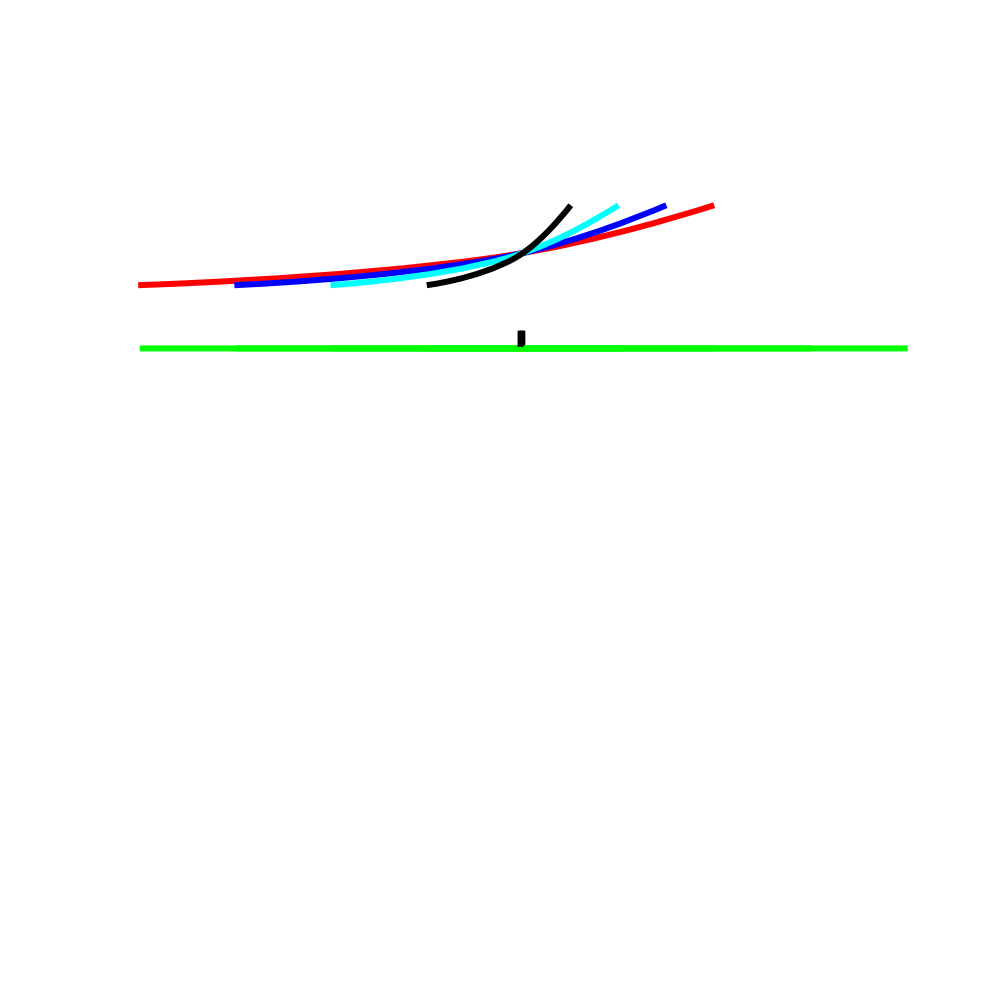
Figure 1 shows the results of a numerical simulation of a turn on a pylon under two different conditions.

Figure 1: Turn on a Pylon

In the no-wind case, the conditions were:

The magenta line shows height as a function of X-position for the no-wind case. You can see that the height is constant.

Also the airspeed is constant, the horizontal distance from the pylon is constant, and the slant range is constant, but these quantities are not represented in the figure.

The horizontal distance can be (almost) anything you choose it to be, but there is only one altitude at which the maneuver will be successful, namely the pivotal altitude. This altitude is shown by the magenta line in figure 1.

2.2  Windy Case

In the windy case, the conditions were:

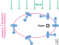
The wind is coming from the north, i.e. coming in from the top of the diagram. The initial position of the aircraft is at the rightmost point of the ellipse. The initial velocity of the aircraft is downwind, i.e. toward the bottom of the diagram.

In the figure,

• The horizontal distance is shown in cyan and the slant range is shown in blue. Both of these are plotted as distance as a function of X-position.
• The required height for the actual maneuver (including wind) is shown in green. Similarly the height for the hypothetical no-wind maneuver is shown in magenta. Both of these are plotted as height as a function of X-position.
• The ground track is shown in black, plotted as Y-position versus X-position. Similarly the pylon is plotted at its X,Y position.

All of these quantities are expressed in units of meters.

Note that the magenta line crosses the green line at X=0, i.e. when the airplane is either directly upwind or directly downwind of the pylon and headed directly crosswind. This is exactly what we expect from the nifty formula, equation 11.

The spreadsheet used to produce this figure is at http://www.av8n.com/fly/turns-on-pylons.xls or http://www.av8n.com/fly/turns-on-pylons.gnumeric

The pattern is an ellipse, with the pylon at one focus. The pattern is not centered on the pylon. When headed downwind you are relatively close to the pylon, and when headed upwind you are relatively far from the pylon.

The long axis of the ellipse extends in the crosswind direction. The wind does not cause the pattern to be “blown downwind” but rather to be shifted sideways, across the wind.

When there is any nonzero wind, the pattern cannot be flown at constant altitude. The altitude is highest when you are headed directly downwind, and lowest when you are headed directly upwind.

For more about all this, see http://www.av8n.com/how/htm/maneuver.html#sec-on-pylons

3  Scaling Arguments

3.1  2D Scaling

Consider the following scenario: we keep the wind the same and keep the airspeed the same, but fly four different-sized versions of the turns-on-pylon maneuver, as shown in figure 2. aAssuming we always enter downwind, we choose four different entry points at four different distances from the pylons. The figure shows a side view of the maneuver.

Figure 2: Different-Sized Turns on a Pylon

How do we fly the maneuver? We can figure it out using a very simple scaling argument, the sort of scaling argument that goes back to Day One of modern science, i.e. 1638. Galileo made good use of scaling arguments, and they have been central to physics ever since.

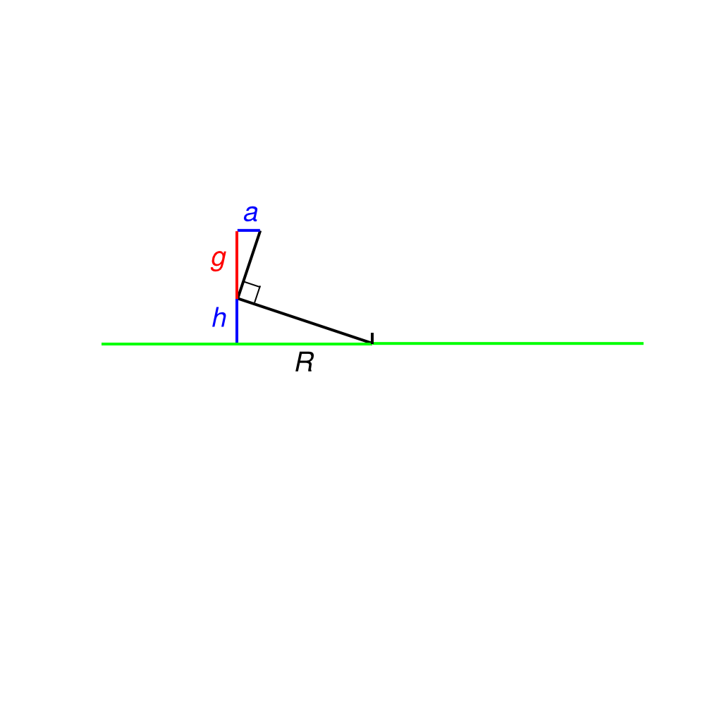
The argument goes like this: We assume the airspeed stays the same, and the wind stays the same. Then if you want to fly a 2x bigger pattern, you need 2x less acceleration at each point. You achieve this quite easily if you fly the same altitudes at corresponding points in each version, because the 2x bigger pattern gives you 2x less acceleration, automagically by the law of similar triangles, as shown in figure 3.

Figure 3: Acceleration versus Height and Distance

To repeat: The scaling law is simple: For any given airspeed and windspeed, the shape of the ellipse does not change. It does not become rounder or pointier. That is, its eccentricity stays the same. To fly a bigger pattern, keep the shape of the pattern the same, keep the airspeed the same, and fly the same altitudes at corresponding points.

To be specific, if we want to scale things by a factor of X:

• times scale in proportion to X.
• horizontal distances scale in proportion to X.
• speeds scale like distance/time i.e. independent of X.
• vertical heights are independent of X.
• accelerations scale like distance/time/time i.e. inversely proportional to X.

3.2  3D Scaling

We now consider another way of scaling the problem. This time we require the height (h) to scale by a factor of X, along with the size of the ground track (x and y).

This is easy in the no-wind case. We just let the speeds scale like the square root of X, in accordance with the pivotal altitude formula. Overall, that gives us:

• Distances scale like X. This includes height as well as horizontal distances.
• Speeds scale like √X.
• Times scales like distance/speed, i.e. like √X.
• Acceleration scales like distance/time/time, i.e. independent of X.
• Bank angles scale like acceleration, i.e. independent of X.

Things are not so simple in the presence of wind, because if you arbitrarily decide to fly a scaled-up pattern, you cannot require the wind speed to change in proportion to your scaled-up airspeed.

In the usual case where you wish to scale up your airspeed but the wind speed is not scaled up, there is no valid scaling. The pattern changes shape. Corresponding points do not exhibit corresponding behavior.

On the other hand, if we play the game the other way around, and let the wind speed determine the scale factor (or the square root thereof), you can fly a scaled pattern. The scale factors are the same as in the no-wind case, as itemized above.

4  How the Numerical Modeling is Done

4.1  Preliminaries

First we derive the equations of motion. This is an exercise in physics and algebra. Some key steps in the derivation are discussed in section 5.

We then wish to solve the equations of motion.

Before we can get very far with this, we need a few key items that are considered "givens", i.e. given by specifics of the situation we are trying to model. The main pilot-oriented givens are the initial aircraft position, initial aircraft velocity, and wind velocity. There are also some internal, technical givens, such as the size of the time-step.

In the example spreadsheet, the wind is from the north, i.e. blowing in from the top of the diagram. The aircraft initial velocity is southbound, i.e. downwind. The initial position is at the rightmost point of the ellipse.

Feel free to experiment by changing the givens and seeing what happens. Hint: things you are invited to change are in cells with a green background.

The main work of solving the equations of motion involves integrating them step by step, as a function of time. This is also known as time-stepping the equations of motion. Yet another name for this is Euler’s method, although we employ some clever tricks to make our calculation much more accurate than the usual first-order Euler calculation.

In the "integration" part of the spreadsheet, each row corresponds to one step in time. Time proceeds top-to-bottom down the spreadsheet. There are just under 800 time-steps.

We assume constant airspeed. That is usually a good approximation. The approximation is improved if your turns on pylons are not overly tight turns, so the required climbs and descents are reasonably gradual. The approximation is also improved if you fly at a high airspeed (high compared to V_y) so that small changes in airspeed produce a large change in altitude in accordance with the law of the roller coaster. You can of course improve the approximation even further if you open the throttle a little whenever you are climbing and close it a little whenever you are descending ... but this is extra work and is not a required or expected part of the maneuver.

We choose to make this assumption because it makes doing the calculations easier, and also because it makes checking the calculations very much easier. This assumption is nontrivial in the sense that a real-world pilot could fly the manuever using some non-constant airspeed profile. For now our simulator is required to fly at constant airspeed. This restriction could be lifted without too much additional work.

4.2  Each Timestep

On each row in the integration part of the spreadsheet, the logic proceeds left-to-right across the spreadsheet, as we now discuss.

In this discussion, the words "new" and "current" refer to quantities available at the current time, i.e. quantities available on this row. In contrast, the word "old" refers to quantities available on the previous line. The expression "even older" refers to the line before that.

1. We start by calculating the new current velocity through the air, V_air, which is a vector. The airspeed is the scalar |V_air|.

   On every row except for the first and second rows, V_air is calculated using first-order Euler with a stride of 2, based on the old acceleration and the even older V_air velocity.

2. We calculate the velocity over the ground, V_gnd, which is a vector. The groundspeed is the scalar |V_gnd|. This is calculated based on the new current V_air and wind velocity vector W (which is a constant, independent of time). This is just simple addition. The wind triangle tells us:

   Vgnd = Vair + W

   (1)

3. We calculate the new current position vector. On every row except the first, we use second-order Euler with a stride of 1, based on the old position vector, the old V_gnd, and the old acceleration vector.
4. We calculate the new current altitude. This is based on the nifty equation 11 as derived in section 5.
5. We calculate the new current acceleration. This is based on the current position and current proper altitude, in accordance with equation 9. This is just trigonometry.

At this point, we have everything we need in order to compute the next row. But as discussed in section 4.4, we will calculate some spinoffs before we move on.

4.3  Exceptions

The exceptional cases are handled as follows:

1. For the purposes of this paragraph, let us restrict attention to columns where Euler calculations normally take place. In these columns, obviously the first row must be an exception. Therec can be no Euler calculations in the first row, because there is no previous data to base them on. Therefore in these columns, the cells in the first row must be filled by initial condition data, i.e. givens.
2. The velocity column has a problem in the second row (as well as the first). For all rows beyond the second row, we use first-order Euler with a stride of 2, but we cannot use stride=2 in the second row, because there is not sufficient older data. We are stuck with stride=1.

   Using stride=1 with first-order Euler gives less accuracy than we would like, so in this special case we use second-order Euler for the velocity. To do this, we need V_air (the velocity), a (the first derivative of the velocity), and ȧ (the second derivative of the velocity). Note that a is the derivative of V_gnd as well as the derivative of V_air. Similar words apply to ȧ. To calculate the latter, we use the fact that at this special point, the entry point, the airplane is headed directly downwind, and is located at the end of the ellipse closed to the focus. It is a property of ellipses that this part of the ellipse coincides with a circle centered on the focus. This is exact to second order. Now for a circle, we know how to calculate ȧ.

   R   =   (given)      →   Vgnd   =   ω ∧ R      ↓   a   =   ω ∧ Vgnd      ←   ȧ   =   ω ∧ a      ↑

   (2)

   That is, for a circle, each time we take the derivative, the direction of the vector rotates 90 degrees, and the magnitude picks up another factor of ω. Here ω is equal to V_gnd/R. Note that we calculate ω in terms of V_gnd/R not V_air/R, even though we are going to use the resulting ȧ to timestep the equation for V_air.

   The second-order Euler calculation is accurate to a small fraction of 1 ppm.

   Here we are using a combination of classic numerical methods, classic mathematics, and dirty tricks. Using second-order Euler is a classical numerical method. Knowing that an ellipse agrees with a circle at this special point is classical geometry. Knowing how to differentiate a vector that is rotating around a circle is classical calculus. The final trick involves exploting a special property of the initial condition; if we entered the pattern at any other point this trick would not work so easily.

   If you want a more generally-applicable trick, for instance if you wanted to enter on a heading that was not directly downwind (or upwind) you might try something more sophisticated than first-order Euler, perhaps a predictor-corrector step.

   In case you are wondering why we don’t use second-order Euler in every row of the velocity column, the answer is that we don’t know how to accurately calculate ȧ except at one or two special points.

4.4  Checks and Spinoffs

In addition to the quantities discussed above, which are needed so that the integration can proceed from row to row, we calculate some additional quantities. This includes numerous checks on the accuracy. It also includes quantities of interest to the customer, including horizontal range and slant range.

As always, we assume coordinated flight, so the heading vector is parallel to the V_air vector.

The accuracy checks include:

1. The heading vector and the position vector should be perpendicular. The angle by which they are off-perpendicular is the aiming error, i.e. the amount by which the wing fails to point at the pylon. The calculated aiming error is on the order of a thousandth of a degree or less, which strongly suggests that my equations of motion are correct, and that the numerical integration of the equations is being done accurately.

   This is quite a sensitive test; if you fly the pattern one foot too high or one foot too low (setting the fudge parameter to 0.31 meter) you will notice a big increase in aiming error.

2. We also calculate the angular momentum. Because we are assuming constant airspeed, all forces in the forward/aft direction add up to zero. The only nonzero net force is the horizontal component of lift. This is constrained (by the rules of the game) to be directed towards the pylon. This is what we call a central force problem. If we measure angular momentum, using the pylon as our datum, angular momentum must be conserved. There are no torques. The only force is directed toward the pylon, so it has no lever arm.

   Calculations confirm that angular momentum is conserved within a few parts per million. This is another sensitive indication that the equations are correct and the numerical integration is being done well.

3. We check the norm of the V_air vector, to confirm that it is accurately constant. This is a check that the equations of motion are consistent with the assumption of constant airspeed.
4. We check to see that the ground track is in fact an ellipse. We choose a rough-fit ellipse (not the best-fit ellipse). The axes of the rough-fit ellipse are chosen based on the max and min X and Y values. That suffices to give agreement between the ground track and the chosen ellipse, accurate within a few parts per million. You can see that the residuals are all positive. We could undoubtedly reduce the residuals by choosing a slightly smaller ellipse.
5. We also verify that when the aircraft is flying across the wind, at a position directly upwind or downwind of the pylon, its altitude in the windy case is the same as it would be in the no-wind case. This is illustrated by the magenta open circle in figure 1.
6. The final check is another visual, not numerical check. We check that the ground track closes on itself, as opposed to precessing, spiraling in, or spiraling out. This check is quite informative, and not unduly dependent on the other tests, because there are lots of ways that the ellipse could precess without failing the constant-airspeed check or the constant-angular-momentum check.

5  Derivation of the Nifty Formula

We wish to derive the nifty formula for the altitude required during a turn on pylon in the presense of wind. We will be using the following quantities:

Assumption: We assume constant |V_air| i.e. constant airspeed.

1. The velocity relative to the air, V_air, is perpendicular to R. That is,

   Vair · R = 0              (4)

   This is required by the rules of the game. The heading is perpendicular to R because the wing is pointing at the pylon, and the airspeed vector is parallel with the heading because we require coordinated flight (zero slip).

2. The acceleration a is antiparallel to R. This is required by the rules of the game, since the wing is pointing at the pylon. That means the horizontal component of lift is pointing at the pylon. Meanwhile, all other forces add up to zero in accordance with the constant-airspeed assumption.

   Because a is antiparallel to R, we have:

   a · R = − |a| |R|

   (5)

3. We will be interested in what happens to all these quantities after some time Δt has passed. Time-stepping the equations of motion gives us:

   new Vair   =   old Vair + a Δt    new R   =   old R + Vgnd Δt

   (6)

4. Combining equation 6 with equation 4 gives us the time-delayed version of equation 4:

   (Vair + a Δt) · (R + Vgnd Δt) = 0.              (7)

5. Muliplying out equation 7 gives us:

   0   =   Vair · R                            +  a · R Δt                        +  Vgnd · Vair Δt                 +  a · Vgnd (Δt)2

   (8)

   The first term vanishes in accordance with equation 4. The second term reduces to |a| |R| Δt because of equation 5. The fourth term is negligible in the limit of small Δt.

6. Rearranging the remaining parts of equation 8 gives

   |a| =

   Vair · Vgnd |R|

   (9)

   This tells us the magnitude of the acceleration. The direction is antiparallel to R as mentioned in item (2). So now a is fully determined, since we know its direction and magnitude.

7. As usual, when the aircraft is properly banked toward the pylon, the geometry of the situation is shown in figure 3.

   In this geometry, the law of similar triangles tells us

   |a| =

   h |R|

   g              (10)

8. Combining equation 9 and equation 10 gives us the nifty expression for the required height at any point during a turn on a pylon:

   h =  Vair · Vgnd g

   (11)

   You can readily verify that this reduces to the conventional expression for the pivotal altitude in the no-wind case.

   Additional discussion of the practical significance of this formula can be found at http://www.av8n.com/how/htm/maneuver.html#sec-pylon-wind especially the part following http://www.av8n.com/how/htm/maneuver.html#eq-pivotal-wind