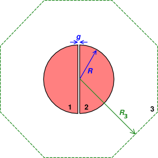
Figure 1: Three-Terminal Split-Sphere Capacitor
Suppose we have N objects, each of which is a piece of conductive material. The ith object has voltage Vi and carries charge Qi
We are going to assume that if we have some charge in a certain equilibrium arrangement, we can (say) double the amount of charge and the new arrangement will also be in equilibrium. This is not true in general, for instance if varactors or other lightly-doped semiconductors are involved, or if the electrodes are free to move (as in a gold-leaf electroscope) … but it is a reasonable approximation for immovable metal electrodes.
Based on this assumption, and on the linearity of the basic equations of electrostatics, we expect that there will be a linear relationship between the charge variables and the voltage variables. We write this relationship as:
| Qi = Cij Vj (1) |
where Cij is called the capacitance matrix. This defines what we mean by capacitance.
On the diagonal, each matrix element Cii is called the self-capacitance of the ith object. Off the diagonal, each matrix element Cij is called the mutal capacitance between the ith object and the jth object.
Let’s consider the simple case where there are only two conductors. They could be, for example, the two plates of an ideal parallel-plate capacitor. For reasons that will be explained later, the full capacitance matrix must have the form:
| C = | ⎡ ⎢ ⎣ |
| ⎤ ⎥ ⎦ | (2) |
In order to make manifest the symmetries of the situation, we define the differential-mode voltage
| ΔV := V2 − V1 (3) |
and the common-mode voltage
| Vc := V2 + V1 (4) |
Inverting these relationships we find
| (5) |
Then we just do the algebra:
| (6) |
So, what have we learned?
For starters, we observe that for each of the two plates, the charge depends only on the differential voltage ΔV and is independent of the common-mode voltage Vc. The insensitivity to Vc is an example of gauge invariance, as discussed in section 1.4
Secondly, we observe that the charge on the first capacitor plate is equal and opposite to the charge on the second capacitor plate. This is a consequence of global charge neutrality, and of the fact that there are no other objects in the universe. Whatever charge appears on object #1 must have been taken from object #2 and vice versa. See section 1.4 for more on this.
Thirdly, as a consequence of these two fundamental physical principles (gauge invariance and charge conservation), as soon as you know one matrix element in a 2×2 capacitance matrix, you know all the others. It’s the world’s easiest sudoku puzzle.
Important caveat: The simple analysis in this section only applies when the two objects have equal and opposite charge. If you are interested in the case of two objects with unbalanced charge, you need to treat it as a 3×3 problem, as discusses in section 1.5.
Terminology: For a two-terminal capacitor, the matrix element b is conventionally called “the” capacitance of the capacitor. It is conventionally denoted C or c. Here we have been calling it b just to avoid confusion with the full capacitance matrix C.
In the case of a parallel-plate capacitor, where the plate area is A and the gap between the plates is g, we have
| b = |
| (7) |
assuming the gap is small compared to the smallest dimension of the plates.
In the case of concentric spheres, we have
| (8) |
Any capacitance matrix must have the following properties:
You can verify that the examples in this section (equation 2 and equation 15) satisfy these requirements.
Let’s turn our attention to the situation shown in figure 1. Object #1 and object #2 are hemispheres of radius R separated by a gap of size g. They are enclosed by a Faraday cage (object #3), represented by an octagon drawn with a dashed line.
We assume the cage is huge compared to the sphere, which is in turn huge compared to the gap. To say the same thing mathematically, we have
| (9) |
We are going to treat this as a three-terminal device. That is, we are going to explicitly account for the charge and voltage on each of the three objects.
To capture the symmetry of the situation, we express the voltages in terms of the following three numbers: V3, Vs, and Va. The mnemonic is s stands for spherically symmetric and a stands for antisymmetric. The meaning of these numbers is defined as follows:
| (10) |
Inverting equation 10 we find
| (11) |
If Vs is zero, then the two hemispheres behave as a parallel-plate capacitor, with
| (12) |
which is independent of V3.
If Va is zero, then we have just a spherical capacitor with total charge Q12, where
| (13) |
which is again independent of V3, except insofar as Vs depends on V3.
Given these expressions for the amount of charge in terms of the voltages, there is a straightforward procedure for finding all the matrix elements of the capacitance matrix. The trick is to differentiate the definition, equation 1. That gives us:
| Cij = ∂Qi / ∂Vj holding constant all Vk except Vj (14) |
It must be emphasized that equation 14 is not the definition of capacitance, but merely a corollary of the definition. It is a rather weak corollary, because if we shift each voltage by a constant (Vj → Vj + shiftj) and fudge each charge by a constant (Qi → Qi + fudgei) then equation 14 cannot tell the difference, even though the physics is different.
Using this corollary, we find that the capacitance matrix takes the form
| C = | ⎡ ⎢ ⎢ ⎣ |
| ⎤ ⎥ ⎥ ⎦ | (15) |
where y = є0πR2/g is the capacitance of a circular parallel-plate capacitor, and x = є04πR is the self-capacitance of a sphere, as we recall from equation 8.
It is even easier to verify equation 15 that it was to derive it. Just plug in some example values for the three voltages and see how the distribution of charge works out.
We recall from equation 9 that R3 ≫ R ≫ g.
Let’s consider the limit where g becomes exceedingly small compared to R. We further assume that R itself is moderately small, and/or Vs=0, so we don’t need to worry about unbalanced charge. Physically, this means the split sphere can be treated as an ideal parallel-plate capacitor, with negligible fringing fields. Mathematically, this means x becomes negligible compared to y, and we can approximate the capacitance matrix as:
| C = | ⎡ ⎢ ⎢ ⎣ |
| ⎤ ⎥ ⎥ ⎦ | (16) |
which has the same meaning (and almost the same structure) as equation 2.
For any particular geometry, is straightforward to calculate capacitances (including mutual capacitances) numerically. The basic idea is to use equation 14, or rather a discrete approximation thereto.
We start by assigning suitable voltages to objects on the potential-grid and observing the induced charge. We find the total charge on each object by summing the cells of the charge-grid occupied by each object.
Then we hold N−1 of the objects at constant potential and wiggle the voltage on the remaining one. We observe what happens to the charge on each and every object by turning the crank on Laplace’s equation. This gives us numerical values for the partial derivatives in equation 14, and therefore numerical values for the matrix elements Cij.
A spreadsheet for doing this, i.e. for solving Laplace’s equation for arbitrary 2-dimensional geometries is discussed in reference 1. (If you don’t like spreadsheets, it would be equally straightforward to solve the problem using a general-purpose programming language such as C++).
Given a system with N nodes, we wish to find the N voltages as a function of the N amounts of charge. In some sense, this is the inverse of the task considered in section 1. Fundamentally, our present task is ill-posed, for multiple reasons:
We have seen that the full capacitance matrix Cij gives the charge values as a function of the voltages, in accordance with equation 1. Alas, this function cannot be inverted. The matrix is singular. Charge conservation guarantees that it is singular. Gauge invariance also guarantees that it is singular.
The best we can do is to write:
| (17) |
where P is called the elastance matrix. Note that the gauge φ is independent of i and j. You are free to choose φ=0, but other folks are free to choose differently. Gauge invariance was built into the capacitance matrix in equation 1, but here we need to handle it separately and explicitly.
The same goes for charge neutrality: It was built into the capacitance matrix, but here we need to handle it separately and explicitly. That is, we demand the following:
| (18) |
Given a capacitance matrix, we can find part of the elastance matrix as follows: Form a diminished capacitance matrix by dropping one row and one column of the full capacitance matrix. Dropping a column corresponds to setting one of the voltages to zero. We can always do this, by fiat, by exercise of gauge invariance. Dropping a row means we are considering the charge on one of the objects to be the designated charge-sink aka counter-electrode. The charge on the charge-sink is a dependent, implicit variable. That is, we have N−1 independent charge nodes and one dependent charge node.
You can choose to drop any one row and any one column. They need not intersect at the diagonal.
Let’s apply these ideas to the split-spherical capacitor as shown in figure 1. Dropping the V3 column and the Q3 row from equation 15, we obtain
| C̸ = | ⎡ ⎢ ⎣ |
| ⎤ ⎥ ⎦ | (19) |
The determinant of C̸ is simply xy, as you can verify by direct calculation. We know that the full capacitance matrix C is always singular, and now we see that the reduced capacitance matrix C̸ also becomes singular when x is zero. This tells us that at this stage of the calculation, we cannot ignore x, which is the self-capacitance of the sphere as a whole. We shall see that x drops out of some of the final results in some cases (equation 21) but not others (equation 22).
In introductory-level discussions of electronics, it is customary to ignore x and similar self-capacitance terms ... but physics tells us that x is always nonzero, and there are plenty of real-world applications where nonidealities such as this must be taken into account.
Using Cramer’s rule or otherwise, we find the corresponding reduced elastance matrix:
| P̸ = | ⎡ ⎢ ⎣ |
| ⎤ ⎥ ⎦ | (20) |
We can check this in the simple case of balanced charge, where Q1=Q, Q2=−Q, Q3=0 for some Q. Then plugging equation 20 into equation 17 we find
| (21) |
so the voltage drop across the capacitor is what it should be, consistent with the familiar expression for a parallel-plate capacitor.
Similarly, we can check the case of completely unbalanced charge, where Q1=Q2=Q/2, Q3=−Q for some charge Q. Then we find
| V1 = V2 = 1/x Q + φ (22) |
as it should be, consistent with the familiar expression for the self-capacitance of a sphere.
In partial analogy to equation 14, we can write
| (23) |
where “floating” means the object’s charge is held constant.
Warning: In fuller analogy to equation 14, it is tempting to differentiate equation 17 to obtain something like:
«Pji = ∂Vj / ∂Qi» floating everything except object i (24a) or simply «Pji = ∂Vj / ∂Qi» (24b)
Equation 24b, if it means anything at all, presumably means the same thing as equation 24a. Alas, equation 24a is complete nonsense, because you cannot hold constant all Qk except Qi, because of conservation of charge (equation 18). You’d be amazed the number of authors who write down something like equation 24b, requiring a change in charge without specifying where the charge is coming from.
Whenever you write down a partial derivative, you should specify the directions. That is, you should specify what’s being held constant and what’s not. Sometimes the directions are obvious from context, but even then it is good practice to specify them anyway.
It is also good practice to carefully distinguish the full capacitance matrix C from the reduced capacitance matrix C̸. Ditto for the full elastance matrix P and the reduced elastance matrix P̸.
Another warning: Comparing equation 23 to equation 14, you might think that on an element-by-element basis, each matrix element of P is the inverse of the corresponding matrix element of C, but this is definitely not true. Note that in the two equations, different things are being held constant.
The energy of the system can be written as
| (25) |
where E(0) is some constant.
Perhaps the easiest way to understand this result, including the factor of ½, is as follows: Suppose we start at zero charge and increase the charge in a symmetrical way, such that
| (26) |
where λ is some abstract dimensionless scalar that goes from 0 to 1. Equation 26 describes a straight-line path in an N-dimensional vector space, where N is the number of nodes in the circuit. We choose this path because it is the simplest way to move charge around without violating conservation of charge. We increase the charge slowly, so we can treat this as an electrostatic situation (not electrodynamic). Then for each λ, the voltages are given by
| (27) |
We can then find the voltage by integrating. Abstractly we can write:
| (28) |
More concretely we can write:
| (29) |
On the last line we have thrown away the term involving φ. It is identically zero, because of conservation of charge, equation 18. This means, among other things, that the constant of integration E0 that appears in equation 25 and equation 29 is not related to the gauge φ that appears in equation 17. That is to say, the gauge of potential energy is not related to the gauge of voltage.
You might be tempted to write something like:
E = ½ Qj Pji Qi + φ ∑i Qi (30a) and then Vk = ∂E/∂Qk floating everything except object k (30b) = Pki Qi + φ
in agreement with equation 17, but that doesn’t work, because of conservation of charge: It is impossible to change the charge on object k without changing the charge somewhere else also. To say the same thing another way, the term involving φ in equation 30a is zero, because the sum is zero, because of charge neutrality.