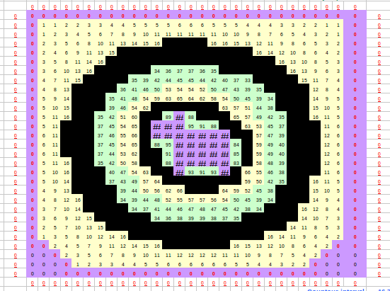
Figure 1: Potential Grid – 2D Cow
I set up some spreadsheets to solve Laplace’s equation, with more-or-less any boundary conditions you want.
The spreadsheet becomes, essentially, a 2D cellular automaton that directly emulates the physics.
This version handles objects in a D=2 universe in rectangular coordinates. In flatland, i.e. D=2, the Z direction simply does not exist. Alas many people are unfamiliar with the laws of physics in flatland. Therefore it might be better to think of this as a D=3 universe in which all D=3 objects are infinitely tall and translationally invariant along the Z axis. In this case, the Z direction exists, but is uninteresting, and the essential physics is the same as the D=2 case. (This is not the same as considering a thin flat “D=2” object embedded in the D=3 universe!) In any case, each cell represents an area dx∧dy in the XY plane. The spreadsheet to handle this case can be found in reference 1.
Occupying a large area near the upper left of the spreadsheet is a grid that I call the potential grid. An example is shown in figure 1. You can set boundary conditions for the problem by choosing cells that you want to represent electrodes, and specifying the potential on these electrodes. For example, reference 1 contains three electrodes:
Within the universe, cells that are not electrodes are called vacuum cells. They contain a formula that will be used to calculate their potential, in accordance with Laplace’s equation, subject to the specified boundary conditions. If you want to “erase” part of an electrode, you should use the copy-and-paste function to fill those cells with the vacuum formula.
Just to the right of the "potential" grid there is second grid that I call the |field| grid because it calculates and displays the magnitude of the electric field at each point. Farther right is a third grid that calculates the charge density (charge per unit volume). If you add up all the cells in a given area, you get a charge per unit length. This means length in the Z direction; it is the charge per unit length of the object rooted in the given area and extending infinitely far perpendicular to the screen.
Principle of operation: Consider a cross-shaped group of 5 elements somewhere on the spreadsheet, and label them as shown in figure 2.
Now the discrete approximation to the second derivative in the horizontal direction is b+c−2w, and in the vertical direction it is a+d−2w. The Laplacian vanishes if w=(a+b+c+d)/4, i.e. if the central element is equal to the average of its four neighbors. Recall we are assuming (d/dz) is zero. This leads to an algorithm that says that for each cell in the vacuum, we want to equal the average of its four neighbors. So the basic step of the algorithm is to run through the grid and just set each cell to the average of the neighboring cells. That does not immediately solve the problem, because whenever we change a cell it requires us to change all the neighbors. However, each basic step brings us closer to a good solution, so we just repeat the basic step several times. This is called the relaxation algorithm.
Another way to motivate the same algorithm is to consider the electrostatic field energy. It depends on the square of the electric field, i.e. the square of the first derivatives of the potential. This energy is minimized when the central cell is equal to the average of its four neighbors. Therefore each step of the update algorithm lowers the local energy.
Tangential remark: You can say that the field energy serves as a Lyapunov function for the relaxation algorithm ... but if this doesn’t mean anything to you, don’t worry about it.
Reference 1 has 841 cells arranged as a 29x29 grid. For a grid of this size, the relaxation algorithm converges in a few seconds. That’s fast enough that it’s not boring, but slow enough that you can observe the propagation of changes if you fiddle with the boundary conditions.
There is a cell just above the top right of the potential grid, labeled object potential. If you change the value of this cell, you can watch how the charge distribution responds.
While the algorithm is running, i.e. after you have changed something but before the algorithm has converged to a solution, the grid contains an approximate solution that doesn’t exactly satisfy Laplace’s equation. That is, during this phase, there will be nonzero charge in the “vacuum”. This is unavoidable; because the spreadsheet strictly enforces local conservation of charge, as discussed in section 2.2. That means there is no way for the objects to acquire the correct charge unless charge flows through the vacuum somehow. The algorithm gradually moves all this charge to the boundaries. The “Manual recalculation” mode (using the “F9” key) may help you observe this, as discussed in section 5. Excel evaluates cells in a sequence that it chooses. The sequence defies simple description, and it has nothing to do with the physics. (Remember, this is an electrostatic problem; there is no physically-significant timescale.) Unfortunately, this sequencing means charge propagates quickly in certain directions across the grid, and slowly in the opposite directions. If you were writing in a computer language that gave you more control than excel does, you could get rid of this unphysical asymmetry by evaluating things in checkerboard-sequence (all the black squares, then all the white squares) or in randomized order.
As mentioned above, just outside the edge of the potential grid is a layer of cells that implement the boundary conditions. In this example, they implement Born/von-Kármán periodic boundary conditions. That is, given a universe of N rows by M columns, row N+1 is constrained to equal row 1, and column M+1 is constrained to equal column 1. You can think of this as a torus, where the top edge of the N×M grid joins the bottom, and the left edge joins the right. Equivalently, you can imagine tiling an infinite region with copies of the N×M grid, subject to the constraint that corresponding cells have the same value in every tile.
Below the potential grid is a graph with many traces; each trace shows the potential as a function of x, while different traces show different y values (rows). Clicking on one of the traces highlights the corresponding row. This may help you locate extremal values.
Below the field grid is a similar graph with many traces.
You can make the universe bigger by adding more rows and columns if you like; use the "fill across" and "fill down" features to propagate the vacuum formula into the new cells. Beware: you must fill from a vacuum cell that is not adjacent to the newly-added cells or the results will be incorrect.
You could extend this calculation to D=3, removing any assumption of translational symmetry. One possible brute-force solution would be to make a spreadsheet with 29 different 29x29 grids and put the appropriately-generalized formula in them. On the other hand, when the problem gets this complicated, you’re probably better off using a more sophisticated programming language, such as C++.
Reference 2 is similar to reference 1, but has several additional features. For one thing, it uses a fancier formula in the vacuum cells. It uses a technique called “over-relaxation” to improve the speed of convergence. This is described at e.g. reference 3.
Basically the idea is to figure out how big a step the simple relaxation algorithm would have‘ taken, and take a step larger than that by a factor of gamma, in hopes of moving more quickly towards the final result. Gamma=1 corresponds to the plain old relaxation algorithm, with no over-relaxation. Values between 1 and 2 make sense. (If gamma were set greater than 2, the electrostatic energy would increase at every step, so the algorithm would not converge.) The value of gamma is controlled by a cell near the top right of the potential grid.
More generally, reference 3 describes a fancy fortran program for doing calculations of this sort. If you’re interested in such things, take a look there.
Reference 2 has another cute little feature, the “gate” cell at the lower right of the potential grid. Setting it to zero sets the vacuum potential to zero everywhere. Setting it back to a nonzero value allows the potentials to be recalculated. This is convenient if you just want to watch how the solution propagates. It is also invaluable for recovering from the following situation: If you enter an invalid expression into a cell in or near the vacuum, the spreadsheet will be unable to calculate the neighboring cell values, and the problem will spread from cell to cell like a disease.
As mentioned above, all the potential grids in reference 1 and reference 2 implement periodic boundary conditions – also known as Born/von-Kármán boundary conditions.
Periodic boundary conditions are not the only possible choice. Another option to have a hall of mirrors. That is, imagine that just to the left of the model universe there is a mirror-image copy of itself. Then impose periodic boundary conditions on the pair (with the appropriate double-length period). Do the same in the vertical direction. You can turn on this feature in the advanced spreadsheet by putting a nonzero value in the cell labeled “hall of mirrors” near the lower-right corner of the potential grid.
The hall-of-mirrors condition has an interesting property: it causes the directional derivative of the potential, in the direction perpendicular to the edge, to be zero at the edge of the universe.
For some applications, for instance if you are trying to model the “self-capacitance” of some object, the hall-of-mirrors boundary condition may approximate the desired physics better than periodic boundary conditions would.
In reference 2, over on the lower right below the main charge-density grid, there is a pair of smallish grids labeled “Charge Conservation”. They serve to illustrate the principle of global charge neutrality and local charge conservation. The pair consists of a potential grid and the corresponding charge-density grid. In this potential grid, you can put an arbitrary arrangement of values in the cells. No matter what you do, no matter how weird the potential-arrangement is, the total charge (i.e. the sum over the charge-density grid) comes out zero, provided you don’t mess with the periodic boundary conditions.
It is easy to see why this must be so: We calculate the charge by convolving the operator (a+b+c+d−4w) with the potential grid. Every nonzero potential cell contributes to the convolution grid five times: once as a, once as b, once as c, once as d, and once (weighted by -4) as w. If you add those five contributions, you get zero every time. (There may be small discrepancies due to roundoff errors, which we ignore.)
The cells in this little grid are just numbers. We do not run the relaxation algorithm on them. This should make it clear that the global charge neutrality, in this model system, has nothing to do with the relaxation algorithm. You could use potential values from the relaxation algorithm, or from some other algorithm, or from a random-number generator, and the total charge in the universe would still be zero. No algorithm can change this zero.
This zero can be seen as a manifestation of Gauss’s law. We can consider the edge of the universe to be a Gaussian pillbox. The periodic boundary condition ensures that whatever field lines leave the top of the universe re-enter the bottom of the universe. Therefore there is no net flux flowing into the universe. (In the example, the field happens to be zero at the edge, making it extra-obvious that there is no net flux.) Since there is no net flux, the net charge on the interior must be zero. The validity of Gauss’s law depends on the structure of the operator (a+b+c+d−4w) and not much else. Its applicability depends on the boundary condition for the universe itself.
Global charge neutrality automatically implies global conservation of charge. Global conservation is vaguely interesting, but it is important in physics, however, to have a local conservation law. Here’s why: Suppose some charge unaccountably disappeared from my lab. It would give me little comfort to be told that it reappeared in some unknowable distant part of the universe; I would be unable to distinguish non-local conservation from from non-conservation. Fortunately, our model system does have a local conservation law. If you increase the potential in any one cell, it causes an increase in the charge-density in the corresponding cell — but this increase is exactly counterbalanced by a decrease in the four neighboring cells (not in some goofy distant cells). Again, this depends on the structure of the Laplacian, not on the update algorithm.
Just below the aforementioned pair of grids is yet another pair of smallish grids, labeled “Gauge Invariance”.
As in most of the other grids, I have imposed Born/von-Kármán periodic boundary conditions. As before, this exhibits global charge neutrality and local charge conservation.
This grid is set up to make it easy to demonstrate the concept of gauge invariance. That is, if you add a uniform constant to all cells, the distribution of charge is unchanged and the electric field is unchanged. Note the contrast:
| If you change the potential of only one cell, the fields are changed, and the distribution of charge is changed; only the total charge is unchanged. | If you change the potential of all cells equally, nothing changes in the field distribution or the charge distribution. |
It is amusing to first prove the gauge invariance property for the N×M universe with periodic boundary conditions, and then let N and M become exceedingly large. That provides a nice way to describe a large universe without requiring any funny boundary conditions that might require gauge-non-invariant amounts of charge “at the edge of the universe”. The torus has no edges.
The Laplacian we have been using – (a+b+c+d−4w) – is manifestly gauge invariant because adding a constant to all cells of a solution produces another solution to Laplace’s equation, and both solutions have the same charge distribution.
In section 2.2, we concluded that the structure of the Laplacian guaranteed local conservation of charge. Here we just concluded that the same structure guarantees gauge invariance. These are two quite different conclusions, but they are profoundly related. Gauge symmetry necessarily implies conservation of charge. Actually this is just the tip of the iceberg; there is a deep and beautiful result called Noether’s theorem that says for every continuous symmetry, there is a corresponding conservation-of-something law. Examples include:
If you want to estimate how much capacitance of your system would have in a very large universe, it is nice to compare the various boundary-value options: grounded enclosure, ordinary periodic boundary conditions, or hall-of-mirrors boundary conditions. In the limit where the boundary becomes very far away from the other circuit elements, the latter two converge to the same limit. The grounded enclosure option does not generally converge to the same limit, as is obvious from the following:
Using any of the aforementioned spreadsheets, if you have just one object and nothing else, the capacitance of the object is always zero. Gauge invariance guarantees it. That is, you can put any potential you like on the singleton object, and it won’t develop any charge. The only way to produce a charge is to have two (or more) objects with different potentials. (The enclosure, if present, counts as an object like any other. There is nothing special about the enclosure.)
I created another very-similar spreadsheet that solves Laplace’s equation in D=3 for objects with rotational symmetry about the Z axis. It can be found in reference 4.
Unlike the previous versions, it does not assume translational invariance along the Z axis, so you can calculate the behavior of objects shaped like pears, or bowls, et cetera. Each cell represents an area dr∧dz in polar coordinates. Note that I am avoiding the word “cylindrical” because mathematicians use the word to describe anything with translational invariance, while physicists use the same word to describe anything with rotational invariance. Sigh.
This is the same as the previous spreadsheet, but it uses the formula for the Laplacian in polar coordinates as discussed at e.g. reference 5.
The potential grid represents a slice through the axis of symmetry. Rotational symmetry implies that any such slice has reflection symmetry. If you fill in the left half-plane of the potential grid (with your chosen objects and other boundary conditions), the spreadsheet formulas will mirror it in the right half-plane. It is not necessary or desirable for you to manually change anything in the right half-plane.
Similar remarks apply to the symmetry of the charge-density grid; it represents a slice through the axis of symmetry.
In D=3 with rotational symmetry about the Z axis, the Laplacian is (d/dr)2 + (1/r)(d/dr) + (d/dz)2; we know the phi-derivative is zero.
(You can contrast this with the previous cases, namely D=3 with translational symmetry in the Z direction, where the Laplacian was (d/dx)2 + (d/dyf)2; we knew the Z-derivative was zero.)
In the cells of the spreadsheet, I have simplified the formula by observing that (1/r)(d/dr) is equal to (1/x)(d/dx) on the slice of interest, by cancellation of a factor of sign(x).
In this spreadsheet there is a fourth grid, just to the right of the grid that shows the charge per unit volume. It shows the charge per unit area (dr∧dz) in a ring. You can find the total charge on an object by summing the numbers in this grid. There is no point in summing the numbers in the charge-per-unit-volume grid; that doesn’t make sense for several reasons, including dimensional analysis.
To improve the accuracy, I use a smart estimate of the quantity (1/r)(d/dr). In particular, I take the arithmetic mean of the left-hand difference (w−b)/x1 and the right-hand difference (c−w)/x2; this accounts for an important nonlinearity because the radius is different in the two denominators.
Validity checks: I verified that a region with a log(r) potential produces zero charge density, with high accuracy. I also checked that the field calculation and charge calculation are automatically gauge invariant, because of the structure of the Lapacian operator.
I implemented periodic boundary conditions in the Z direction, and this is the default behavior. I also implemented hall-of-mirrors boundary conditions, which you can optionally use instead.
In the R direction, there is only one choice: the perpendicular component of the electric field vanishes on this boundary. This is reminiscent of the hall-of-mirrors boundary condition, but there is no physical interpretation in terms of tiling the universe. Instead, this can be viewed as surrounding the region of interest, at each Z level, with an annulus extending to infinity. The potential on this annulus depends on Z but is independent of R. This means that outside the region of interest, there will be zero charge, although there will be nonzero fields. These fields seem a bit unphysical. To make these fields go away, you can arrange that the potential at the large-R boundary is independent of Z. To achieve this, it suffices to arrange that one of your electrodes fully encloses all the other electrodes.
You can use these spreadsheets to calculate capacitance.
We start by assigning suitable voltages to objects on the potential-grid and observing the amount of induced charge. We find the total charge on each object by summing the cells of the charge-grid occupied by each object.
Then we hold N−1 of the objects at constant potential and wiggle the voltage on the remaining one. We observe what happens to the charge on each and every object by turning the crank on Laplace’s equation. This gives us numerical values for the matrix elements Cij.
For details on what a capacitance matrix is, and how to calculate its matrix elements, see reference 6.
The following remarks apply to all three versions of the spreadsheet.
I’ve got “iteration-mode” turned on.
Suggestion: If you are going to seriously play with this, you will want to make use of the spreadsheet’s recalculation controls. You might want to delay recalculation if you are making numerous changes to the grid, but thereafter you will want automatic recalculation:
At any time you can invoke the manual "recalculate now" function with the F9 key.
The following small features probably require having the “1997” (or later) version of excel. They are known to work with version 9 (the one that comes with office 2000):
