Figure 1: Kelvin Probe
To answer various questions that come up from time to time:
| (1) |
where x(,) designates the charge of the first object when contact-electrified against the second. It is even possible to have two objects D and E such that
| (2) |
A related but easier-to-visualize piece of physics is this: given fixed terminals (A1 and A2) made of absolutely identical material (A) plus a moving part of type B, I can create a generator (e.g. as shown in figure 3) which uses contact electrification to move charge from A1 to A2 at a steady rate. Does that imply that A ranks above B and below B in the so-called triboelectric series? I don’t think so.
Mostly it’s just a combination of everyday things:
The idea of work function is central to any understanding of electrochemistry, including contact electrification (aka static electricity) as well as batteries, fuel cells, electroplating, et cetera. Please make sure you are familiar with the ideas in reference 1 before continuing with this document.
Let’s build a simple parallel-plate capacitor, i.e. two plates sitting hear each other, nothing else. One plate is made of Fe (work function 4.63 eV) and the other is made of Ni (work function 5.2 eV). In equilibrium, the two plates will differ in voltage by ΔV = 0.57 volts. We believe, for reasons to be discussed later, that equilibrium is established by exchange of electrons.
As usual, the capacitance is
| C = є0 |
| (3) |
where A is the plate area, and g is the gap between them.
If the gap g is very small, there will be a huge capacitance. We know the capacitance, and we know the voltage, so we can calculate the charge on the capacitor,
| Q = C ΔV (4) |
If we pull the plates apart while allowing the plates to remain in equilibrium, the charge Q will be a decreasing function of the gap-size g, in accordance with equation 3. The voltage ΔV remains constant.
Now, if we have a constant voltage and the capacitance is changing, the charge will be changing, in accordance with equation 4. This changing charge means a current must be flowing through whatever is responsible for maintaining the two plates in equilibrium.
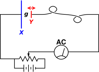
This is the central idea behind the Kelvin probe, as shown in figure 1, which is used to measure the difference in the work function of two materials. (This is sometimes called a Kelving bridge, but beware that there is another quite different circuit that is also called a Kelvin bridge.)
The blue capacitor plate X is made of one material, and the red capacitor plate Y is made of another material with a different work function. The red plate is connected to the rest of the circuit via a flexible wire. The red plate is forced to move back and forth horizontally at a fairly high frequency. This causes the gap g to change.
Let’s start by ignoring the potentiometer. That is, we move the slider all the way to the left, so the potentiometer voltage is zero. Then the wiring simply serves to keep the two capacitor plates in equilibrium, by allowing rapid exchange of electrons. In equilibrium, there will be an electric field E in the gap. The total voltage drop E·g will be equal to the difference in the work functions between the two metals, i.e. the difference in electron chemical potential.
| (5) |
As always, there will be a charge on the face of each capacitor plate. The surface charge density will be proportional to E. The total charge will therefore be proportional to area, proportional to the work-function difference, and inversely proportional to g.
When we change the gap, there must be a change in charge. That means a current flows in the circuit. This is observed on the AC current meter.
As a refinement, we can use the potentiometer to make this a null measurement. That is, we slide the potentiometer to the point where we observe no AC current. The null condition is reached when the potentiometer voltage is just equal to the difference in work functions. The two plates are being held in the non-equilibrium situation where there is no electric field in the capacitor gap.
We can use an ordinary DC voltmeter (not shown in the diagram) to read out the voltage on the potentiometer (in the null condition) and call that the result of our measurement of the difference of work functions.
By making the red electrode Y relatively small, the apparatus can be used to probe the work function as a function of position on the surface of object X. Instruments to do exactly this are sold commercially.
Now let’s consider a slightly different scenario. The plates are in equilibrium, but the process that established equilibrium is no longer operating effectively. That is, the plates are insulated. The charge on each plate is constant. If we now pull the plates apart, the voltage ΔV will grow in proportion to the gap.
To repeat: There is a huge difference between pulling the plates apart at constant voltage (which implies decreasing charge) and pulling them apart at constant charge (which implies increasing voltage).
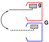
We can apply what we know to build a powerful static electricity generating machine, as shown in figure 2.
The blue compartment is made of one material and the red compartment is made of another material with a different work function. There also exists a shuttle, shown in black. For definiteness, you can imagine it has a work function intermediate between the other two, but in fact it doesn’t matter; the shuttle work function will drop out of the calculation.
To operate the machine, the shuttle, which has a long insulating handle, is first touched to the inside of the red compartment. This touching brings the shuttle into equilibrium with the red compartment. There is a modest voltage across an infinitesimal gap, which means a huge charge in accordance with equation 4.
Next we withdraw the shuttle. As it moves away from the wall of the compartment, for a while it will remain in equilibrium. There will be field emission, and if the device is operated in air there will be corona discharge, all acting to keep the two objects in equilibrium.
But at some point these processes will stop. In air, corona discharge requires a field on the order of a few megavolts per meter. For a one-volt difference in work function, that corresponds to a gap of less than a micrometer. When the gap is bigger than that, there is no longer any way for equilibrium to be maintained.
Let’s be clear: for very small gaps, there is equilibrium and constant voltage. For gaps larger than a micrometer or so, there is constant charge – the charge is “frozen” onto the shuttle.
We now move the shuttle to the other compartment and follow the same procedure. The shuttle will pick up a different charge, because of the difference in materials.
By shuttling back and forth, we can transfer a constant amount of charge per cycle. We soon develop a huge potential difference across the gap G between the compartments.
|
Note that the shape of the compartments is meant to serve as something
of a Faraday cage, so that the fundamental charge-transfer operation
is not affected by the huge potential across the gap G. That means the machine is not limited by breakdown across the small gap g, but only across the large gap G, which you can make as large as you want. |
This is a nice refinement, in contrast to poorly-engineered or non-engineered contact electrification situations (such as sliding your shoes across a rug in winter) where the generated field can nullify the fundamental charge transfer, much as the potentiometer nulls out the work-function difference in the Kelvin probe. |
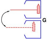
An interesting variation of this machine is shown in figure 3.
The odd thing about this machine is that the two compartments are made of the same material.
This time it is necessary for the shuttle to be made of a material with a different work function. Also, the shuttle has a tricky shape.
The trick is that in one compartment, you choose to use the broad face of the shuttle to make contact with the compartment. Therefore, when you pull the shuttle away, at the time the charge becomes frozen onto the shuttle, there will be a big capacitance because of the big area, in accordance with equation 3.
Then, in the other compartment, you choose to use the very narrow point of the shuttle to make contact. So, at the time the process of equilibration ceases and the charge becomes frozen onto the shuttle, the electric field is about the same and the voltage difference is about the same as in the previous case, but the charge is much less, in proportion to the area.
By shuttling back and forth, you can move a more-or-less constant amount of charge per cycle.
Please keep in mind that chronology is not history. The actual history is incomparably more complicated. For a survey of early work, see reference 2. Some highlights include:
We now close our study of electricity and magnetism. In the first chapter, we spoke of the great strides that have been made since the early Greek observation of the strange behaviors of amber and of lodestone. Yet in all our long and involved discussion we have never explained why it is that when we rub a piece of amber we get a charge on it, nor have we explained why a lodestone is magnetized. You may say, “Oh, we just didn’t get the right sign.” No, it is worse than that. Even if we did get the right sign, we would still have the question: Why is the piece of lodestone in the ground magnetized? There is the earth’s magnetic field, of course, but where does the earth’s field come from? Nobody really knows — there have only been some good guesses. So you see, this physics of ours is a lot of fakery — we start out with the phenomena of lodestone and amber, and we end up not understanding either of them very well. But we have learned a tremendous amount of very exciting and very practical information in the process!
In the early 1980s, I discussed the physics of contact electrification with Feynman, and it was news to him at that time. The point of this item is that you shouldn’t believe everything you read in books. Just because Feynman didn’t know about it doesn’t mean “nobody” did.