Figure 1: Ground State of a Harmonic Oscillator
Coherent states (including Glauber states) are elegant and very helpful for understanding what goes on in oscillating systems, including harmonic oscillators as well as many kinds of waves. They show us the correspondence between quantum oscillators and classical oscillators. Among other things, they make it clear that even in fully quantum mechanical systems, not everything is quantized, not all waves are quantized, not all states are discrete, et cetera.
If some of this comes as a surprise to you, you are not alone. A lot of smart people have gotten this wrong over the years. Indeed, the guy who figured this out the first time got the Nobel prize; see reference 1.
If you want some basic background on how to think about quantum states, see reference 2 and reference 3.
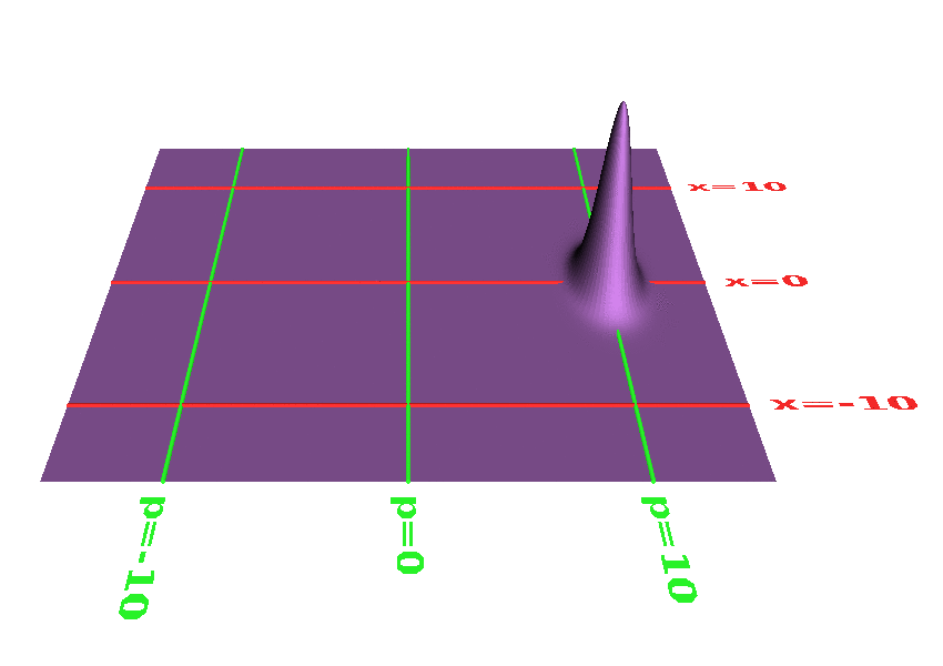
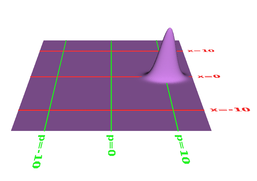
The ground state a harmonic oscillator is shown in figure 1. It is centered at the origin in phase space. As you can see, it has a certain RMS width in the x direction ... and also a certain nonzero width in the p direction. To keep things simple, we have chosen units of mass and time so that the standard deviation comes out to be 1.0 in each direction.
The ground state – like everything else in this universe – upholds the laws of quantum mechanics. It also upholds the correspondence principle, in the following way: This diagram corresponds to a harmonic oscillator such as a mass on a spring, with the mass sitting at its equilibrium point, not actually oscillating. The laws of quantum mechanics tell us that if we are only interested in momenta and distances that are large compared to the size of the ground state, that corresponds to zooming out from figure 1, whereupon the coordinates of the oscillator are sitting still, highly concentrated at the origin in phase space.
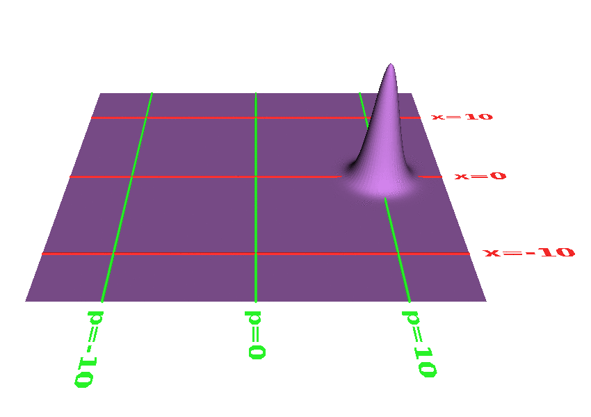
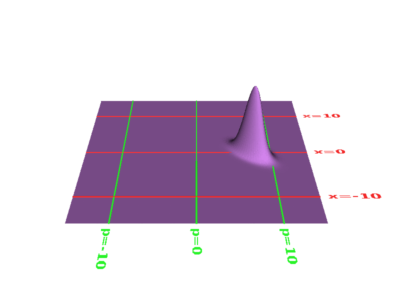
Another state of the harmonic oscillator is shown in figure 2. This is called a coherent state, also known as a Glauber state.
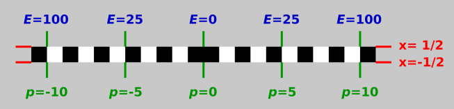
Each and every Glauber state is congruent to the ground state. That is, the shape is identical. The x-coordinate of the center of the coherent state oscillates back and forth at an angular frequency ω0, the resonant frequency of the oscillator. The p-coordinate of the center also oscillates back and forth at the same frequency, 90 degrees out of phase with the x-coordinate. Combining these two oscillations gives us a circle in phase space, as shown in figure 2. (More generally, it might look like an ellipse, but you can always choose units so as to make it a circle.) In this example, the amplitude of the oscillation – the radius of the circle – is 10, in units where the standard deviation of the ground state is 1 unit, as before.
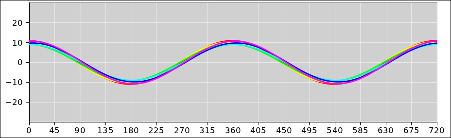
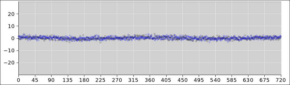
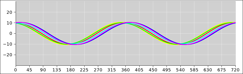
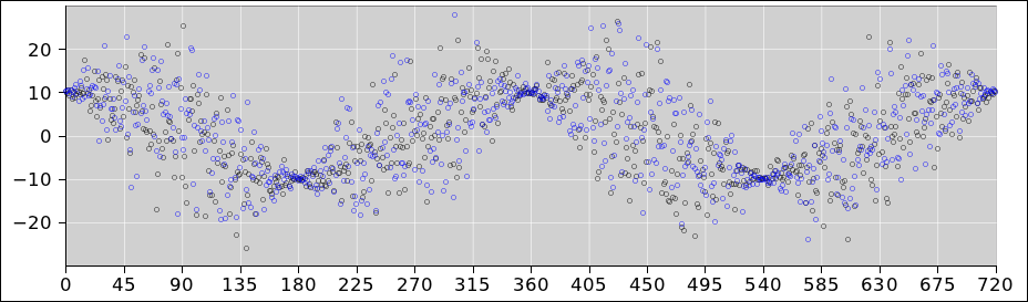
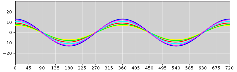
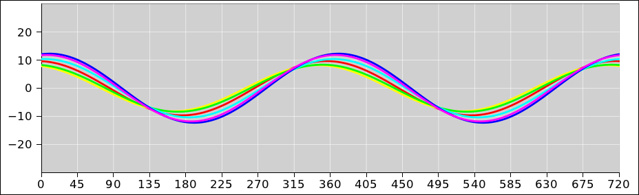
This coherent state upholds the laws of quantum mechanics, of course. It also upholds the correspondence principle, in the following way: This diagram corresponds to a harmonic oscillator such as a mass on a spring, with oscillating back and forth, and the expected frequency, with an amplitude equal to 10 times the standard deviation of the ground state. The waveform is shown in figure 11. The six curves represent six points on the probability distribution, each one standard deviation from the center.
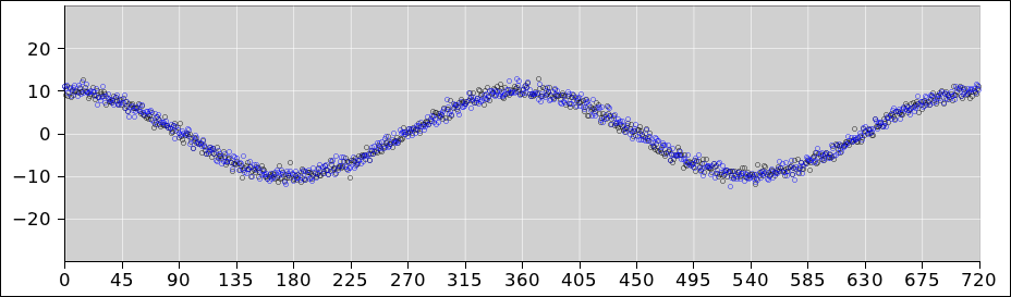
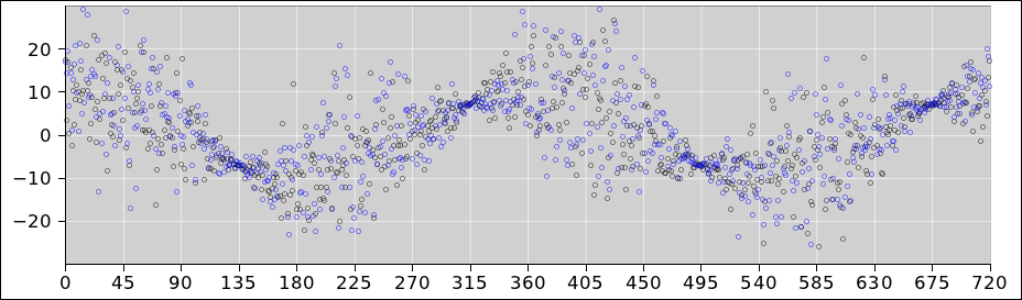
The scatter plot shown in figure 12 is a more faithful representation of the same thing, just not as pretty. Here is the physics: We create a coherent state at time t=0. We let it evolve for some amount of time t, and plot the phase ω0t as the abscissa. At the time t we measure the x-component. That is, we project our state state of definite position. We plot this as the ordinate, as one one dot in the plot. We then prepare another copy of the coherent state and repeat the experiment, to obtain another dot. We need to prepare a new state each time, because the measurement process destroys the state. That is to say, the scatter plot is based on an ensemble of coherent states. The problem with the nice-looking curves in figure 11 is that they could be interpreted as representing the time-evolution of a single state (rather than an ensemble), which would be quite wrong.
The quantum mechanics tells us that if we increase the magnitude of the oscillation by a large factor, and zoom out accordingly, what we see is a particle oscillating with the expected frequency at the expected amplitude. In relative terms, all the probability is highly concentrated at the expected location. The absolute width of the distribution stays the same, but it relatively small compared to the large amplitude.
Note the following important contrast:
|
Do coherent states uphold the laws of quantum mechanics? ... Yes! |
Are they discrete? ... No! Are they quantized? ... No! |
You can construct a coherent state anywhere you like, anywhere in phase space. Pick any real number x and any real number p, and then create a coherent state that is centered at the point (x, p) at time t=0. It will return to that point once per cycle, as we see for example in figure 2.
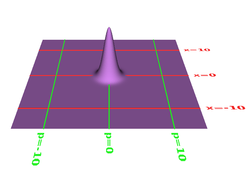
The ground state itself can be considered a coherent state located at the point (p, x) = (0, 0).
Let’s be clear: Integers are quantized; real numbers are not. You can put a coherent state anywhere you like, with a center position specified by two real numbers, (x, p). Figure 5 shows a state similar to figure 2, except with a much smaller amplitude (namely 0.5 standard deviations rather than 10).
Here are the corresponding waveform and scatter plot:
The topic of coherent states is relevant to harmonic oscillators of every kind, including mechanical oscillators, electronic oscillators, and everything else. For example in an electrical LC oscillator, rename the coordinate x to be q (the charge on the capacitor) and rename the momentum p to be φ (the flux in the inductor). Then all the rest of the equations are the same. The laws of classical physics guarantee that if you choose q as your coordinate, φ is the dynamically conjugate momentum. When in doubt, ask the Lagrangian. The Lagrangian knows all and tells all.
This topic is also relevant to waves in linear media, including electromagnetic waves, ordinary sound waves in air, and the waves traveling along a piano string. These systems are linear to a good approximation under normal circumstances (although any system will become nonlinear if you push the amplitude high enough).
Everything we have said about oscillators applies to waves, because each standing-wave mode of the wave field can be considered a separate oscillator.
We therefore conclude as follows: Not all light is quantized. Not all waves are quantized. Not every oscillator state is quantized. A lot of people who ought to know better keep getting this wrong, but the facts remain as I have stated here.
We can make even stronger statements about all systems, not just harmonic oscillators and linear waves: Basis states are not the only states. Even if the basis states are quantized, there is a continuum of other states, namely linear combinations (aka superpositions) of two or more basis states.
Technical note: Strictly speaking, these phase-space diagrams show the Wigner function. You can convert to/from the Wigner representation to the more familiar position-basis representation by means of a Weyl transformation.
| For present purposes, the Wigner function can be interpreted as the probability density in phase space. | In general, the Wigner function can take on negative values, so it cannot be interpreted as a classical probability. |
| Every quantum-mechanical state can be represented by a corresponding Wigner function. | You can cook up distributions in phase space that do not correspond to any legitimate quantum-mechanical state. In particular, a very narrow distribution would violate the Heisenberg uncertainty principle. |
| Quantized states are an abstraction. They exist in theory. They sometimes play a useful role in theoretical calculations. | They do not exist in practice. Nothing in the real world is really quantized. |
| In theory, the stationary states of an undamped harmonic oscillator are quantized. | In practice, all oscillators have some damping. |
| Some folks point to the existence of sharp spectral lines as evidence for stationary states. | Spectral lines are not infinitely sharp. The width is proof that the states are not actually stationary. |
| A stationary state, by definition, exists for all time. | No state that you can actually construct is a stationary state. It would not be necessary or possible to construct such a thing, because it exists for all time. |
|
In theory, an ideal harmonic oscillator has certain stationary states. These are standing waves. These are the photons (for an electrodynamic system) or the phonons (for a mechanical system). (The photons we are talking about here are harmodons – not wave packets, as explained in section 6.) These are not the only states, but they form a sometimes-convenient set of basis states. They are one possible set of basis vectors in an abstract, high-dimensional vector space.
Let’s be clear about the contrast:
| The photons are states. | They are not the only states! |
| The photons collectively can be used as a basis set. | They are not even the only possible basis states! |
| Sometimes it is convenient to use the photon representation. | Sometimes another representation is more convenient. |
| Photons have quantized energy. | Many other states (e.g. coherent states) don’t have quantized energy or quantized anything else. |
Quantum mechanics was born out of thermodynamics, and the two subjects remain intimately connected. For example, entropy is basically a measure of area in phase space, measured in units where the ground state has unit area. More specifically, entropy scales like the logarithm of the area, so the ground state has zero entropy, as it should. Each coherent state is congruent to the ground state, and also has zero entropy.
To do anything fancy with modern thermodynamics i.e. statistical mechanics, you need to sum over area in phase space. This includes summing over all the dimensions in a high-dimensional space. The conventional and reasonable way to do this is to project the state-vector onto some set of mutually orthogonal basis vectors, and then sum over the basis set. So, you commonly see something called the partition function, denoted Z, which takes the form of a sum over states. Indeed the letter Z stands for “Zustandssumme”.
Now, it must be emphasized that Z is not a sum over all states, but rather a sum over the basis states. Often it is convenient to use the photon basis, but this is not required. Absolutely any basis will give the same answer.
Consider for example a so-called two-state system, such as the spin of an electron. That doesn’t mean the system has two states; it means the system has two basis states, in any particular basis. There are infinitely many ways of choosing a basis. Sometimes you prefer one basis and sometimes another, as discussed in reference 4. Furthermore, even if you have settled on a particular basis, there are uncountably many non-basis states.
For a harmonic oscillator, there are countably many basis states in any particular basis. There are uncountably many different ways of choosing a basis. Furthermore, even if you have settled on a particular basis, there are uncountably many non-basis states.
The set of all Glauber states is not a basis, because the states are not mutually orthogonal. You can see that the state shown in figure 5 has a tremendous amount of overlap with the ground state. We say the set is overcomplete.
We can speak of the Glauber state representation even if it is not a basis.
You can of course express any coherent state as a linear combination of basis states, using the photon basis or any other basis. In second-quantized language, there is a particularly elegant representation of the coherent state in terms of creation operators. The details can be found in reference 5 or reference 6.
In this system, you have a choice of what to measure, as is usually the case in any quantum mechanical system.
As always, you can change from one representation to another, at some cost:
For example, suppose you prepare a state of definite energy E, i.e. a state of definite photon number, i.e. one of the basis states in the photon representation. It has zero entropy. If you now project that on the Glauber state representation, you are guaranteed not to get a single Glauber state. (For simplicity, we are ignoring the obvious exceptional case where you started out in the ground state and remain in the ground state.) However, it is unlikely that the new state will have either |q| or |φ| values that differ very much from √E.
Conversely, suppose you prepare a coherent state and then project it onto the photon basis. You are guaranteed (with one obvious, trivial exception) not to get a state of definite energy. You will get a superposition of photon states. If you measure the energy, you will get a distribution of results. The entropy of this distribution nonzero. (Even though projecting onto a new basis is reversible, measurement is irreversible, so that accounts for the increased entropy.) In any case, it is unlikely that the energy eigenstates that make significant contributions to the new state will have energies that differ very much from q2 + φ2.
If we ask about the energy of just one of the theoretical photon basis states, it will be discrete; it will be quantized. However, when we look at a real state in a real system, it will be a superposition of basis states, and the expected value of the energy ⟨E⟩ will not be quantized.
As another way of looking at things, reference 7 presents an interesting animation. It can show a coherent state oscillating back and forth, while also indicating how the photon basis states combine to create the coherent state. It can also show the basis wavefunctions separately. (Beware that the vertical axis of the animation is somewhat overloaded, in that it is used to portray both energy and probability density.
In this section we discuss the meaning of Planck’s constant qualitatively, at a level consistent with phase space diagrams such as figure 2. A deeper discussion can be found in section 3.4.
| Planck’s constant ℏ is the natural unit for measuring area in phase space ... much as the radian is the natural unit for measuring angles. In this context, the word “action” is sometimes used to denote area in phase space, so we can say Planck’s constant is the natural unit for measuring action. | You may have heard h or ℏ referred to as “the quantum of action”. This is (at best) a misnomer, since phase space is not actually quantized ... just as angles are not quantized. |
| This idea applies to a wide range of systems, including not just harmonic oscillators but also anharmonic oscillators, free particles, spin systems, et cetera. |
| Planck’s constant is the amount of area per basis state in phase space. | Again, this does not mean that phase space is discrete; it just means that if you find N states with less than Nℏ of total area, they will not be linearly independent. |
| This means that if you are choosing a basis, you should choose a discrete set of basis states. This gives us a natural reason for choosing some discrete basis. | This does not mean that phase space is naturally discrete, for at least two reasons: (a) there are infinitely many different ways of choosing a basis, and (b) once you have chosen countably many basis states, there are uncountably many other states. Uncountable is a whole lot bigger than countable. Basis states are not the only states! |
Planck’s constant also appears in important expressions such
as
and
|
This does not mean that energy is quantized or that momentum is quantized. For example, in figure 8 the energy levels are quantized and evenly spaced but the momentum is not quantized at all, whereas in figure 9 the momentum is quantized and evenly spaced, but the energy is not evenly spaced. |
Also, beware that the quantum-mechanical frequency ω that appears in equation 1 cannot be determined by means of the correspondence principle, because it is typically not the system’s classical frequency ω0, for reasons discussed in section 4.2. (For example, if you add energy to a satellite orbiting the earth, the orbital frequency ω0 goes down.)
You may have heard h referred to as “the quantum of energy”, but that idea has numerous serious problems, as we now discuss, in hopes of suppressing some common misconceptions.
Equivalently, as discussed in section 4.2, you can sometimes write E = (N+½)ℏω0, where N is called the photon number. That means ℏ could be considered the energy per photon per unit frequency, provided you are only interested in the theoretical energy eigenstates, and only interested in perfectly harmonic oscillators.
Let’s be clear: Without changing the frequency of oscillation, you can add energy to the oscillator by increasing N, the number of photons.
This is important, because the laws of quantum mechanics apply to everything in the universe, not just harmonic oscillators. We need to think about things clearly, so we don’t make assumptions that get us into trouble when we encounter coherent states, nonlinear systems, et cetera.
Note the contrast:
| Harmonic Oscillator | Everything Else |
| For harmonic oscillators (and for waves in linear media, which is essentially the same thing) the same set of circles in figure 8 can be used to explain “equal area per basis state” and/or “equally spaced energy levels”. The two ideas cannot easily be separated. | For anything that is not a harmonic oscillator, the idea of “equal area per basis state” remains valid and important, but the idea of “equally spaced energy levels” does not survive. An example is shown in figure 9. |
As you can see in table 1, there are at least three different ways in which the idea of discrete, equally-spaced energy levels can break down:
Table 1 should make it clear that the idea of equally-spaced energy levels is something of a fluke. It only works for harmonic oscillators, and not necessarily even then.
| Simple | Damped | ||||||||
| Harmonic | Harmonic | Particle | 1/r | ||||||
| Oscillator | Oscillator | in a Box | Potential | etc. | |||||
| Equal area in phase space ... | |||||||||
| stationary states: | Yes | Yes | Yes | Yes | Yes | ||||
| all pure states: | Yes | Yes | Yes | Yes | Yes | ||||
| Equally spaced in energy ... | |||||||||
| stationary states: | Yes | No | No | No | No | ||||
| all pure states: | No | No | No | No | No |
| It is important to know about harmonic oscillators and photons. | We should not assign harmonic oscillators more importance than they deserved. In particular, we should not allow them to foist a perverted notion of quantization on us. |
| A lot of things in this world can be modeled as simple harmonic oscillators. | A lot of important things are not even remotely harmonic, not even remotely linear, and not even remotely undamped. |
In section 3.3, we noted that Planck’s constant ℏ is the natural unit of measure in phase space, much like a radian is a natural unit of angle.
This analogy is really quite close. More specifically, Planck’s constant can be seen as a conversion factor, converting action to phase, namely the quantum mechanical phase Φ mentioned in section 4.2. Quite literally, h converts action to phase (measured in cycles) while ℏ ≡ h/2π converts action to phase (measured in radians).
In this way, quantum mechanics reduces to the classical principle of least action via the method of stationary phase. This is profoundly analogous to the way physical optics reduces to geometric optics.
The quantum mechanical phase Φ can be observed directly in situations where one part of the wavefunction interferes with another, such as in a two-slit interference experiment. The propagation of a free particle can be understood in these terms, via a Huygens construction, which is in effect a “many slits interference” experiment. If you carry these ideas to their logical conclusion, you wind up with the path integral formulation of quantum mechanics. See reference 8.
The path integral formulation provides the clearest way of seeing the connection between quantum mechanics and thermodynamics. Roughly speaking, thermodynamics can be seen as the analytic continuation of quantum mechanics, in much the same way as the method of steepest descents is related to the method of stationary phase. It’s the same idea, with or without a factor of i in the integrand.
States that differ enough in phase will be linearly independent. The value of Planck’s constant tells you how much action it takes, i.e. how much area in phase space it takes to accomplish that. This is crucial when you are trying to construct a basis set.
As mentioned in section 2, in the Glauber state representation, the correspondence between quantum oscillators and classical oscillators is simple and direct.
In contrast, in the photon representation, the correspondence is much more complicated and much more indirect. Indeed, starting from the photon representation, usually the best strategy is to convert to the coherent-state representation and invoke the correspondence principle from there.
For example, when the electric company sells you electricity, they are not selling you a photon state. To a much better approximation, they are selling you a coherent state centered at q = q′ cos(ω0t+θ), for some phase θ. The amplitude q′ is on the order of 110√2 or 220√2 volts, and the quantum mechanical uncertainty Δq′ (i.e. the halfwidth of the state) is many many orders of magnitude smaller. Indeed, the quantum fluctuations are negligible compared to other fluctuations in the waveform.
There is widespread confusion about the important equation E = ℏω. The quantum-mechanical frequency ω that appears here is the rate-of-change of the quantum-mechanical phase Φ. It is not the classical frequency of oscillation ω0.
In fact, ω = (N+½)ω0. That is to say, in the N-photon state, the quantum-mechanical phase goes around and around at a rate approximately N times greater than the classical oscillation frequency. Specifically, we can write a multiphoton state as a product:
| (3) |
This corresponds to writing the energy as a sum:
| (4) |
Unlike ω0, neither ω nor Φ has any direct correspondence with the classical physics of a harmonic oscillator. The correspondence principle has got nothing to say about these quantities.
Consider the limit in which the spring constant of the harmonic oscillator goes to zero. We now have a free particle.
In this situation, the thing that most closely corresponds to a coherent state is the famous minimum-uncertainty wave packet. Alas this state does not retain its shape the way a Glauber state does; it gets skewed (i.e. sheared) in phase space, which we perceive as a spreading in the x direction. This stands in contrast to the original harmonic oscillator, where the parabolic potential provides a focusing effect that keesp the wavepacket from spreading. This is why they are called “coherent” states – they stick together rather than spreading out.
Let’s discuss states of definite energy. With a little bit of work, we can portray them in phase space. In figure 8, the border between one color and the next shows where the state is. The border has zero width. The colored regions are not the states; they are the regions between states.
These energy eigenstates are stationary states. In some sense they rotate, just as the coherent states rotate around the origin at frequency ω0 ... but since the energy states are circles, the rotation leaves them unchanged.
The states are equally spaced in energy. Each of the colored rings in the figure has the same area as the others. This stands to reason, since the ring is the area between two energy eigenstates.
Given that the states are equally spaced in energy, where E = x2 + p2, the Nth state must have x and p values proportional to √N. You can see that the 25th state is a circle tangent to the lines of constant x=5 and x=−5. It is also tangent to the lines of constant p=5 and p=−5. By the same token, the innermost color-to-color boundary is tangent to the lines (not shown) of constant x=±1 and p=±1.
These rings are one way but not the only way to divide phase space into cells of equal area. You are allowed but not required to use the photon representation.
Perhaps the simplest example of something that is not a harmonic oscillator is þe olde particle in a box. (In some sense, this can be considered a highly anharmonic oscillator.) The stationary states are simple sine waves. The stationary states are equally spaced in phase space, but the energy levels are not equally spaced – not even close. Specifically, as we go from state to state, the momentum values are equally spaced, but the energy values are not. The energy goes like momentum squared. The color-to-color boundaries in figure 9 indicate the energy eigenstates. Just as in figure 8 the states are equally spaced in area, but the way this happens is quite different.
The following table spells out the spacing and other properties of the Nth state for a harmonic oscillator in contrast to a particle in a box.
| Harmonic Oscillator | Particle in a Box | ||
| state number | N | N | |
| x-extent | ∝√N | constant | |
| p-extent | ∝√N | ∝N | |
| gross area A | ∝N | ∝N | |
| A(N) − A(N−1) | constant | constant | |
| energy E | ∝(x2 + p2) | ∝p2 | |
| energy | ∝(N + ½) | ∝N2 | |
| E(N) − E(N−1) | constant | ∝N | |
Figure 10 shows something we call a squeezed state. It is very similar to an ordinary unsqueezed coherent state, except that its width has been decreased by a factor of s in one direction and increased by a factor of s in the other direction. This leaves its area in phase space unchanged, which makes it easier to understand how this state complies with all the laws of physics, including thermodynamics and quantum mechanics.
You can see from figure 10, or from the corresponding waveform in figure 11, that squeezing allows certain phase-sensitive measurements to be more accurate than the corresponding measurement of an unsqueezed state. In particular, in this state, when |x| is large, x can be measured with relatively little quantum uncertainty. This comes at the price of greater uncertainty in the dynamically conjugate variable, p, as we would expect based on the Heisenberg uncertainty principle. For more about this, see reference 6.
For obvious reasons, figure 11 is sometimes called a “mustache” diagram. Note that for clarity, the waveform diagram uses a greater amount of squeezing than the phase-space plot does (aspect ratio of 10 versus 2).
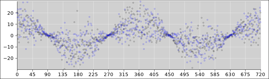
Figure 13 shows a coherent state that has been squeezed in a different direction. This state is desirable if you want to determine the value of x when |x| is small, and you want to minimize the uncertainty Δx.
The corresponding waveform is shown in figure 14.
More generally, you can squeeze in any direction, so that the angle between the long axis of the squeezed state and its direction of motion can be anything you choose. An example can be seen in figure 16.
The corresponding waveform and scatter plot are shown in figure 17 and figure 18.
You can also change the amount of squeezing. In the limit where the state has very little uncertainty Δx (and correspondingly great uncertainty Δp) it approaches the ideal “position eigenstate”. You can never make a perfect position eigenstate, but you can come close.
Beware that the term “photon” has two different technical meanings:
Both of these terms are very widely used. There is no point in arguing about which is right or wrong, or even better or worse. They’re just different. Both terms refer to perfectly reasonable concepts.
Constructive suggestion: In situations where confusion is possible, I recommend avoiding the word “photon” entirely. You can use the term harmodon to describe concept (a), and use the term wave packet to describe concept (b).