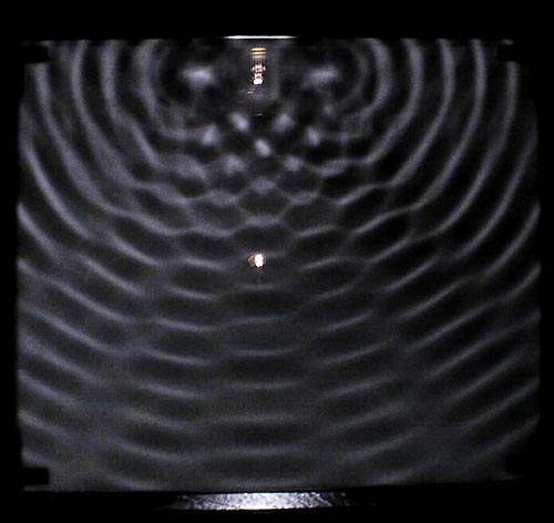
Figure 1: Ripple Tank Apparatus at Claremont
Models and Pictures of Atomic Wavefunctions |
There are various ways of modeling and/or depicting atomic wavefunctions. You can use waves in a pool of water, as discussed in section 2. You can also use Chladni patterns and waves on a string, as discussed in section 7. You can also use pictures, including animated pictures and animated scatter plots, as discussed in section 9, section 13, and section 14. Many other folks have done animations over the years, including reference 1.
Simple mathematics and simple models represent some (but not all!) of what happens in real atoms, as discussed in section 5 and section 6.
The term “orbital” is often used in this context, but it is somewhat ambiguous; for details on this, see section 8.2. For some general background on how to think about quantum states, see reference 2.
In general, the bigger the better, as discussed in section 2.2, but this demo works even on a small scale. You can do it as a classroom demo, with one container per student, or perhaps one for every two students.
I have a huge number of plastic tubs, 15 cm in diameter and 12 cm high. Originally, they came from the store with 1.5 lbs of crumbled cheese in them. I wash them and save them, because they are super-handy. If you don’t have such things, you can carry out the wave demo using ordinary bowls. Disposable styrofoam soup bowls are adequate. The cheese tubs are nicer, because they are taller and hence less likely to spill.
Fill each container about half way. Add a drop of dish detergent (e.g. Dawn or Lemon Joy) and make a few bubbles, so that it is easy to see what the surface is doing.1
For a tub or dish of water, excite the motion by pushing some smallish solid object up and down, displacing some of the water. I have a collection of empty pill bottles that I use for plungers.
Another way to create a |2p+⟩ wavefunction is to combine |2px⟩ and |2py⟩ excitations together, with a quarter-cycle phase lag between them.
The |2s⟩ wavefunction for a pool of water is profoundly analogous to the |2s⟩ wavefunction for an atom.
The demo in section 2.1 can be scaled up to larger and larger containers.
As the container gets larger, you may need a larger plunger, but otherwise you can do all the experiments listed in section 2.1. Soap bubbles are not needed for the larger sizes.
For the swimming pool, you use yourself as the plunger. The instructions in this case are slightly different:
This is the |2s⟩ wavefunction for the pool of water. It is profoundly analogous to the |2s⟩ wavefunction for an atom.
Let that wave die away, then ....
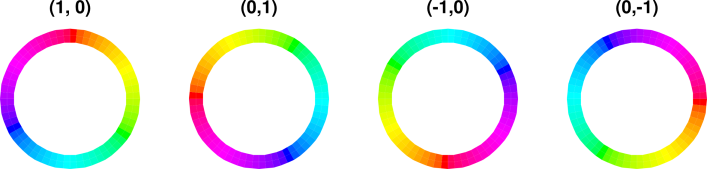
This is the |2px⟩ wavefunction.
Let that wave die away, then ....
This is a simple experiment, but it is important for a number of reasons.
In a two-dimensional system such as the water surface, you can construct infinitely many wavefunctions in the |2p⟩ family, but if you have more than two, they will be linearly dependent. For instance, you can readily convince yourself that the |2p+⟩ wavefunction is a superposition of |2px⟩ and |2py⟩ with a particular phase. Similarly the |2p−⟩ wavefunction is a superposition of |2px⟩ and |2py⟩ with the opposite phase.
| (1) |
You can easily go the other way, writing |2px⟩ as a superposition of |2p+⟩ and |2p−⟩. That is to say, the set {|2px⟩, |2py⟩} is not the only possible basis. Another perfectly good basis is the set {|2p+⟩, |2p−⟩}. Innumerable other basis sets are possible.
This gives us a complete description of the N=2 shell. In two dimensions, there are no other linearly-independent patterns that can be formed with only one node.
In three dimensions, there would be one more pattern. The obvious “rectangular” basis in D=3 is {|2s⟩, |2px⟩, |2py⟩, and |2pz⟩}. Another often-useful basis is {|2s⟩, |2p+⟩, |2p−⟩, and |2pz⟩}. As always, there are infinitely many other bases.
Recall that for ordinary vectors, such as position vectors or momentum vectors, we need two basis vectors to span a two-dimensional space, and three basis vectors to span a three-dimensional space. The wavefunctions in the N=2 family are vectors in an abstract four-dimensional space. This can also be called a function-space and/or a Hilbert space.Terminology: It is common for people to say that in three dimensions, there are only four orbitals in the N=2 shell (namely one s-orbital and three p-orbitals). This is, alas, an abuse of the terminology. There are infinitely many different possible orbitals, i.e. infinitely many possible wavefunctions in the function-space. The thing that we should be counting is not the number of wavefunctions but rather the dimensionality of the function-space. So when somebody says there are “four orbitals” you have to translate: What they really mean is that four basis wavefunctions suffice to span the space.
There is a tremendous amount to be learned by observing what goes on in a ripple tank. Running waves, interference, diffraction, refraction, reflection, et cetera.
Another good demo involves waves on a string. You want both the tub-of-water demo and the string demo. The provide complementary information, in the following sense:
| For the string (to be discussed in this section), the abscissa of the wavefunction is one-dimensional while the ordinate is two-dimensional. The ordinate can be described as having two different polarizations. | For the tub of water (as discussed in section 2), the abscissa of the wavefunction is two-dimensional while the ordinate is one-dimensional. The polarization is not interesting and is usually not mentioned. |
| The genuine quantum wavefunction for a single particle has a three-dimensional abscissa (in real space) and a two-dimensional ordinate (in its own somewhat abstract space). Neither the string model nor the tub-of-water model suffices by itself, but by using both models you can piece together a much more complete picture. |
Technical details: Ordinary household string is not optimal. You want something heavy as well as flexible. The beaded chain that they use for pulling the switch on overhead lamps is one possibility. Helical “telephone cord” is another possibility; the helical design makes it especially flexible. An extra-long Slinky is another possibility; such things are sold just for this purpose. Highly-flexible rope is another possibility. In all cases, longer is better. For simplicity, I will refer to all of these media as “strings” but the word “string” must not be taken literally.It helps to fasten the ends of the string to sturdy supports – perhaps clamp stands or some such – but if you’re in a hurry you can just have students hold the ends.
On the string, the polarization vector is two-dimensional. You can start by creating horizontally-polarized waves and contrasting that with vertically-polarized waves. Then you can move on to circularly-polarized waves, such as are seen on a jump-rope. You can launch the waves by hand. If you want to get fancy, you can use an electric egg-beater or a variable-speed electric drill; chuck up some sort of wheel and attach the string off-center. Install a swivel (available from the fishing-supplies store) to decouple the undesired "spin" aka "twist" from the desired "orbital" motion.
Choose a rotation rate that is slow enough that people can follow the actual motion with their eyes. A long rope with lots of sag – i.e. no unnecessary tension – will give you relatively many nodes at a relatively low frequency.
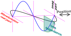
Figure 3 shows an example of a circularly polarized standing wave on a string. In a one-dimensional situation like this, there is only one quantum number. We will use the spatial frequency ξ to specify the state. This stands in contrast to a three-dimensional atom, where there are three quantum numbers, conventionally N, l, and m. The state in figure 3 is the |ξ=±1⟩ standing wave. It can be constructed as a superposition of |ξ=+1⟩ and |ξ=−1⟩ running waves.
It must be emphasized that in the string model, the string is whirling around and around like a jump-rope, not merely up and down; see section 4.4 for an explicit animated depiction of this. The whirling motion gives us a good model of the time-dependence of the phase of the wavefunction, as it rotates in the complex plane. The blue curve shows the wavefunction at an early time, and the black curve shows the same function one quarter-cycle later.
| Examples: Rotating Ordinate | Examples: Non-Rotating Ordinate |
| The circular polarization of the string makes an important point about the time-dependence of the wavefunctions in an atom, and about the symmetry of the ordinate. Consider a particular point on the string: in a rotating standing wave (as used in a jump-rope game) the chosen point remains at a fixed distance from the axis as it goes around and around. The wavefunction can go around from +X to +Y to −X to −Y and back to +X without ever crossing through zero. | In the tub of water, the polarization vector is uninteresting because it is one-dimensional; a one-dimensional vector looks a lot like a scalar. That is, the water moves from “up” to “down” or equivalently from “plus” to “minus”. Also note that a scalar cannot go from plus to minus without crossing through zero. As such, the water is not a good model of quantum mechanics. Sometimes you can label the lobes of a QM wavefunction as “plus” and “minus” – but sometimes you can’t ... and even if you can such labels are likely to be misunderstood. |
| It is true that at any given time, each lobe of the |ξ=±1⟩ wavefunction in figure 3 is -1 times the other lobe. However, this is not a complete description, and runs the risk of being misunderstood. | In ordinary two-phase house wiring, the black phase is -1 times the red phase and vice versa. Unlike quantum mechanical wavefunctions, the voltages do not go around and around like a jump-rope; each phase simply goes up and down, crossing through zero twice per cycle. |
| Any discussion of the wavefunction in terms of “+” and “−” is not just misleading, it is also very incomplete, because it cannot even begin to describe what is going on in an atomic |2p+⟩ or |2p−⟩ orbital. For more on this, see section 13. |
Note: In quantum mechanics – and everywhere else – a two-component vector can be represented as a complex number (and vice versa). You can use either representation, or both, at your convenience.
The string can demonstrate standing waves as well as running waves.
The other option is to use an assistant to hold the far end of the string (while you hold the near end). Start out with the string taut and straight, with both persons moving their hands in unison. This is an |s⟩ wave. Then you speed up for a time, while the other person keeps steady pace, so that you advance the phase at your end by 2π relative to the other end. Then continue in unison again. The result you are trying to achieve is shown by the blue curve in figure 5.
For this demo to work, the far end of the string cannot be attached to a fixed point. The end of the string needs to move, so that the string can do F·dx work. You can’t have energy flowing in the wave unless there is something at the far end to absorb the energy.
Figure 4 shows an animation of a running wave packet. The packet can be described as a sinusoidal carrier modulate by a Gaussian envelope.
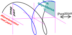
Figure 5 shows a snapshot of the |ξ=+2⟩ running wave on a string. As mentioned in section 4.2, at any particular location, the string is whirling around and around like a jump-rope (not merely up and down). The blue curve shows the wavefunction at an early time, and the black curve shows the same function one quarter-cycle later. See section 4.4 for an explicit animated depiction of the whirling motion.
Note that unlike in figure 3, there are no nodes in figure 5. The ordinate of the wavefunction never goes to zero. Indeed it never goes anywhere near zero.
Also note that unlike in figure 3, there is a definite direction of travel in figure 5. The wave works like an Archimedes screw, carrying energy and momentum in the direction marked “Position” in the figure. The time-dependence of the wavefunction (radians per unit time) tells us about the energy density (ℏω), while the space-dependence (radians per unit length) tells us about the momentum density (ℏk). The ratio dω/dk tells us about the velocity. (Note: as always, the wavenumber is given by k = 2πξ.)
Even though the wavefunction in figure 5 has the same magnitude at all times, it is still a running wave, not a standing wave. Such a wave carries a steady flow of energy and momentum. The ordinate is a vector, and looking at its magnitude doesn’t tell you everything you need to know. There are things – such as the momentum operator – that act on the vector as a whole, not on the magnitude. The momentum operator is relevant here, because the things I’m calling running waves (figure 5) have nonzero momentum, while the standing waves (figure 3) do not.
For more yet another model of running waves, see section 13.
The message of figure 3 and figure 5 can be made easier to grasp with the help of interactive animated computer graphics.
In the middle row of the table, note that the |ξ=−1⟩ wavefunction has a negative spatial frequency. It has the symmetry of a left-handed screw, whereas positive frequencies have the symmetry of a right-handed screw.
Some people may be able to look at these diagrams and learn learn all there is to learn that way. However, for most people I recommend doing the actual experiment. Get a friend and a rope and do the experiment. Treat these diagrams merely as instructions for what to do and what to look for. Among other things, you will discover that the running wave “feels” different from the standing wave. The person at one end of the running wave is doing positive work, while the person at the other end is doing negative work.
The computer animations are a simpler and cleaner than experiments with a real rope. Among other things, the real rope is affected by gravity, by centrifugal force, and by aerodynamic drag in ways that make things more complex than one might like.
This one-dimensional model (using rope or computer) is in some ways analogous to what goes on in an ordinary three-dimensional atom ... and in some ways not. The analogy is however indirect and quite abstract, and the details are beyond the scope of the present discussion. In other words, don’t worry about it. More importantly, though, there are one-dimensional systems in nature. For example, in many cases, to a first approximation, a dye molecule can be considered a short one-dimensional electrically-conducting wire. The models presented in this section give an excellent description of the wavefunctions for electrons on such a wire.
These are in some sense four-dimensional diagrams: They show the real and imaginary parts of the ordinate of the wavefunction, as a function of one spatial coordinate (x) and as a function of time. Time is represented by time itself, via the animation. Note that the true physics of a hydrogenic atom is six-dimensional; for simplicity we are restricting attention to situations where the spatial y and z dependence is irrelevant.
If you know a little about wave mechanics, we can use it to shed some additional light on what’s going on. Otherwise you can skip to section 6.
Let’s consider what the wavefunction looks like right near the edge of the pool. Using polar coordinates (r, φ) in the plane, we can ask about the wavelength in the azimuthal direction, i.e. the dφ direction, i.e. the direction that goes around the circumference. One complete trip around the circumference must correspond to an integral number of wavelengths; otherwise the wavefunction would not be single-valued, i.e. it would not be a function at all. The defining property of |p⟩ family of wavefunctions is that they have one wavelength around the circumference (while |d⟩ wavefunctions have two, |f⟩ wavefunctions have three, et cetera). The wave equation gives us two solutions (leftward and rightward propagation, or in this case clockwise and counterclockwise) so there must be exactly two |2p⟩ wavefunctions in two dimensions. We know this just by counting, plus an appeal to symmetry.
Very roughly speaking, you can think about the angular dependence of the |2p+⟩ and |2p−⟩ wavefunctions in terms the Bohr model, i.e. electrons orbiting around the nucleus like planets around the sun. This is wrong in general, but it sometimes serves as a rough first approximation. The approximation gets better and better as we consider waves where more and more wavelengths fit into one trip around the circumference, i.e. as we move up the series |2p⟩, |3d⟩, |4f⟩, et cetera. Note that for each shell (i.e. each principal quantum number) we are talking about the wavefunction with the highest possible angular momentum. These are called Rydberg atoms and have been the subject of intensive study, theoretically and experimentally.
Let us now switch attention to the radial direction, i.e. the dR direction. We can understand the |2s⟩ wavefunction as a standing wave, constructed from a radially-outbound running wave that reflects off the edge of the pool and returns as a radially-inbound running wave. Combining the two running waves gives us a standing wave with one node.
Switching back now from pools (two dimensions) to atoms (three dimensions), we have identified four possible wavefunctions the form a basis for the N=2 shell: |2s⟩, |2px⟩, |2py⟩, and |2pz⟩. No matter what basis we choose, there cannot be more than four basis functions when N=2. It’s just geometry and symmetry and counting. Then the electron spin gives us double occupation of each orbital. That makes eight. Anything else is linearly dependent, or involves a different shell (i.e. different principal quantum number).
This is the fundamental basis for the octet rule as it pertains to individual atoms in the second row of the periodic table, in particular to their ionization potentials and electron affinities. There is something special about having eight electrons around an individual atom. (This must not be taken as an endorsement of anything resembling an octet rule for molecules; see reference 3 for details.)
Maybe you’re not convinced. Maybe you think there ought to be another wavefunction just like |2s⟩ but a little bit different, having one node (so it belongs to the N=2 family) but somehow different, having the node in a different place. Well, sorry, it can’t be done in a high-Q resonant system such as this. (See section 12 for details.) If you attempt it, you won’t be able to satisfy the boundary conditions. Recall we said the |2s⟩ wavefunction could be constructed from a running wave that reflects off the wall of the pool and returns. That only works with one very specific wavelength. If you try it with a slightly different wavelength, it will come back with the wrong phase. The phase errors will accumulate with every bounce. Over the long haul you will get a superposition of waves with all possible phases, which adds up to zero. This is physics: basic wave mechanics. Or you could call it mathematics: Sturm-Liouville theory and all that.
The previous paragraph pretty much answers the question of why atoms have discrete shells. You can’t have something that is halfway between shell N=2 and shell N=3. If you try, you won’t be able to satisfy the boundary conditions.
The picture described so far works for low-numbered atoms, up to and including the second row of the periodic table.
When we consider higher atomic numbers Z (anything beyond neon) and hence higher shells N (the third row of the periodic table and beyond), we need to think much more carefully about the relationship between mathematics and atomic physics. In particular, observation tells us that in terms of physics, i.e. in terms of energy, that shells get filled out of order relative to the naïve mathematical numbering. We are talking about really basic observations here, starting with the existence of transition metals.
The physics is as follows:
The electron’s kinetic energy depends on the curvature of the wavefunction. A high-N wavefunction in a small region will have lots of curvature, hence lots of kinetic energy.
A high-N wavefunction far from the nucleus has an unfavorable potential energy. A high-N wavefunction near the nucleus has an unfavorable kinetic energy. Therefore we expect the small-N shells to fill up first.
For high-Z atoms, once the small-N shells are filled up, things get very complicated. Once we start filling the high-N shells, things proceed in a somewhat peculiar order. This produces transition metals among other things. Hund’s rules and all that.
The first row is easy: There is only one wavefunction, the |1s⟩ wavefunction. It just sits there. No nodes. No dynamics. Electron spin means we can have two electrons in this orbital. So the first row has two members and ends at helium, Z=2.
The second row has eight members and ends when we have filled the N=2 shell (on top of the N=1 shell), namely neon, Z=10.
So far so good.
Things get quite a bit more interesting when we get to the third row. The observed fact is that the third row has eight members and is is complete at argon, Z=18. Here is where we must explain the difference between a chemistry-shell and a mathematics-shell.
The N=3 chemistry-shell (also called valence-shell) is complete when we have filled the |3s⟩ and |3p⟩ wavefunctions (namely argon) ... but at this point the N=3 mathematics-shell is far from complete, because the |3d⟩ wavefunctions haven’t been touched.
There are some things we know about math, some things we know about physics, and some things we know about chemistry. The point here is that mathematics by itself will not correctly explain the chemistry when N=3 or beyond. Physics is needed. A closely related point is that jumping up and down in the pool accurately tells you certain things about the atomic wavefunctions, such as the symmetry of the wavefunctions and the dimensionality of the function-space – but it will not accurately tell you the energy thereof.
The key to understanding the third row of the periodic table is this: the |3d⟩ electrons have a higher energy than the |3s⟩ and |3p⟩ electrons. The |3d⟩ electrons are members in good standing of the N=3 mathematics-shell, but they don’t2 contribute to the N=3 chemistry-shell, because they are energetically unfavorable. So let’s try to figure out why they have a higher energy.
At this point the usual glib explanation is to say that the |3d⟩ wavefunctions have a node at the origin, so the |3d⟩ electrons don’t spend enough time near the nucleus and accordingly have an unfavorable potential energy. The problem is, if you believe that argument, you would predict that beryllium would be a noble gas, because the |2p⟩ wavefunctions also has a node at the origin, so you would think the |2p⟩ electrons would be disfavored3 compared to the |2s⟩ electrons. We need a better argument.
We need to consider more than just the node at the origin. We need to consider what happens in the neighborhood of the origin. For a p-wave, if you move away from the origin, you pick up electron amplitude to first order. For a d-wave, you only pick up amplitude to second order. You have to go a lot farther to get significant amplitude. Also note that the nucleus is heavily screened by the electrons in the lower-N shells, so it’s not simply a question of how close you can get to the nucleus, but rather a question of whether you can get inside the inner shells, i.e. inside the screening.
You can set up some |3d⟩ wavefunctions in the pool of water. The easiest one has the symmetry
                  + +     - -
                  + +     - -

                  - -     + +
                  - -     + +
and has two nodes, straight lines that cross in the middle. The water is fairly quiet in a fairly good-size region near the middle.
To summarize: the key idea is that the |3d⟩ wavefunctions don’t sufficiently get inside the screening, so they have an unfavorable potential energy. Argon would almost always prefer to be inert than to react using a |3d⟩ wavefunction. The same is essentially true of other third-row atoms ... although the |3d⟩ wavefunctions can’t be dismissed entirely, as discussed in connection with SF4 below.
Not only do the |3d⟩ wavefunctions have high energy compared to the |3p⟩ wavefunctions, they even lose out to the |4s⟩ wavefunction in potassium and calcium. But not by much. It is competitive with |4p⟩, which is roughly why the ten fourth-row transition metals are where they are in the periodic table, between calcium (where filling the |4s⟩ subshell is completed) and gallium (where filling the |4p⟩ subshell begins). This placement does not, however, mean that |3d⟩ is necessarily filled before |4p⟩ is begun. Atoms in this part of the table can change their valence by shifting electrons back and forth between |3d⟩ and |4p⟩.
You can set up standing waves on a metal plate. For present purposes, it’s appropriate to choose a round flat plate, supported at the center. Excite it by bowing. Make a heavy-duty bow using the frame of hacksaw or pruning saw, plus high-test kernmantel fishing line or weed-trimmer line. Put rosin on the bowstring ... it’s just like bowing a violin. If you put powder on the plate, it will move to the nodes and remain there, making the node pattern visible. This is called a Chladni pattern.
In a series of four papers published in 1926, Schrödinger presented the Schrödinger equation, and also solved it to find the stationary states – the energy eigentstates – in the special case of a spherically-symmetric potential. See reference 4. There is a separation of variables, such that the solution can be written as a product Rn(r) Ylm(θ, φ), where Rn(r) is a purely-radial function and Ylm(θ, φ) is a purely angular function. The angular part is just a spherical harmonic, as discussed in section 14.
This solution is very nearly a solution for the electron wavefunction in a hydrogen atom. It is not quite exact, because the spin of the proton and electron introduces a small magnetic interaction that makes the problem not quite spherically symmetric. It is traditional to ignore this slight nonideality and call these solutions the hydrogenic eigenfunctions.
There is a general rule (from Sturm-Liouville theory) that says a complete set of eigenfunctions can be used as a basis, and any solution can be written as a superposition of these basis functions.
Let’s be clear about one thing: The hydrogenic basis functions are not the only solutions to the Schrödinger equation. They are not even the only possible basis set. You can choose any basis you like. In each basis set, there are countably many basis functions. You can then write uncountably many solutions, each of which is a superposition of basis functions.
We are faced with two incompatible ideas:
At the next level of detail, (n, l, m) specifies the external part of the wavefunction, while an additional variable is needed to specify the electron spin, which is considered internal to the electron. As a numerical example, the quantum numbers (n, l, m, s) = (2, 1, 1, +½) correspond to the |2p+⟩ wavefunction with the electron in the spin-up state.
These two descriptions are incompatible in the Heisenberg sense. For any given atom, any attempt to ascertain the position will randomize future measurements of the spectroscopic quantum numbers (n, l, m), and any attempt to ascertain those quantum numbers will randomize the future position.
This isn’t as much of a problem as it could be, if we have a large supply of identically-prepared atoms. We can measure one atom, throw it away, measure another atom and throw it away, and so forth. By collecting enough such measurements, we can gradually work out what positions are consistent with which spectroscopic quantum numbers (or vice versa). A program that does this is discussed in section 9.
So far, we have explained how the spectroscopic quantum numbers (n, l, m, s) apply to an atom with only a single electron. The remarkable thing is that the same general ideas and much of the terminology can be extended to multi-electron atoms. The resulting wavefunctions won’t be exactly the same, but they will be sufficiently similar that we can use the same terminology. In particular, the solutions will have the same symmetry. As an example, let’s compare the |2s⟩ electron in lithium to the |2s⟩ excited state in hydrogen. The radial part of the wavefunction Rn(r) will differ as to details, but in both cases it will have n−1 nodes (i.e. 1 node, since n=2 in this example). Roughly speaking, this is called the independent electron approximation – but beware there are several different approximations that go by that name.
The word “orbital” is often used, especially in the chemistry literature, but it is somewhat ambiguous.
This is awkward because a level is not the same thing as a state, especially if there is degeneracy or near-degeneracy involved.
I don’t recommend such a narrow definition, because the choice of basis is a choice. You can choose whatever basis you like, but others may choose differently. The choice is just as arbitrary in quantum mechanics as it is in introductory vector analysis. Energy eigenfunctions are not the only possible functions ... or even the only possible basis functions. You can use the sp3 functions as basis states if you want, whether or not they are stationary states.
In the rare situations where the distinction matters, you can probably figure it out from context.
Note that to solve the equation of motion for a two-electron atom, the solution must be a function of eight variables. We can write something like Ψ(x1, y1, z1, s1, x2, y2, z2, s2), where x, y, and z are external (spatial) variables and s is an internal (spin) variable. In contrast, a single-electron wavefunction such as φ(x, y, z, s) cannot – by itself – solve the equation of motion for a multi-electron atom. By itself, it does not even have the right functional form. By itself, it is not even a basis function for the multi-electron atom, because we cannot write the solution as a sum of single-electron orbitals. That is, we cannot write
| (2) |
or anything like that. Instead, the simplest thing that makes sense is a sum of products:
| (3) |
To repeat: In equation 3, the basis functions are not single-electron orbitals, but rather products of such orbitals.
This sort of sum-of-products representation is tremendously useful, for the following reason: It is relatively easy to draw a picture in two dimensions. Visualizing the structure of a fully three-dimensional object is much more difficult. Visualizing something in an abstract six-dimensional (or eight-dimensional) space is virtually impossible for most people. The physics does not require you to write the wavefunction as a sum of products, but you can understand why people are usually happier talking about single-electron orbitals rather than the full multi-electron wavefunctions.
Constructive suggestion: A dye molecule can be roughly approximated as short wire, extending in one dimension only. The one-electron orbitals in such a system are functions of one variable. A two-electron wavefunction can be written as a sum of products, where each term is two-dimensional, i.e. a function of two variables. That’s something we can draw pictures of. An interesting example of this can be found in reference 5.
You can’t live in a brick, but you can live in a house made of bricks. Similarly, you cannot solve the multi-electron equation of motion using a one-electron orbital by itself, but you can solve it using a wavefunction made of a sum of products of such orbitals.
I cobbled up a javascript applet that collects data from 10,000 simulated atoms to demonstrate how position data can be extracted from hydrogenic eigenfunctions, for specified spectroscopic quantum numbers. At present, the applet only deals with the |1s⟩, |2s⟩, and |2px⟩ basis wavefunctions.4 Push the appropriate Go button.
Note that this uses Javascript as opposed to Java, which means there are far fewer security issues.
This applet makes somewhat aggressive use of new Javascript language features. If your browser does not support these features, instead use the older stand-alone Java version in reference 6. You can download the source file, read it to verify that the Java cannot possibly do anything nasty, compile it, and then run it.
The scale bar in the lower left corner has length a0, where a0 is the Bohr radius, namely
| (4) |
The scale bar gradually turns from red to black, serving as a progress meter.
Credit: The idea of using an animated scatter plot to show the probability density for an atomic wavefunction is an oldie but a goodie. I got it from a film somebody (possibly PSSC?) made in the 1960s, back when using computers to make educational animations was a lot more exotic than it is now.
Chemistry straddles the quantum/classical boundary:
| With rare exceptions, it is possible and useful to make classical ball-and-stick models of what atoms and/or ion cores are doing. | It is never possible to make a good classical model of what the electrons in an atom are doing. Electrons in this situation are highly quantum mechanical. |
Electrons weigh 1836 times less than protons, and it matters. It means that electrons will be highly quantum mechanical under conditions where anything heavier than a proton can be considered classical. In particular, the conditions I have in mind involve atomic length-scales, chemical energy-scales, and ordinary non-cryogenic temperatures.
Also note that any basis wavefunction other than the |1s⟩ wavefunction will have one or more nodes. A node is a place where the probability density goes to zero. The node in the |2s⟩ basis wavefunction is a sphere of radius 2a0. The node in the |2px⟩ basis wavefunction is the plane located at x=0.
It would be particularly hard to make a ball-and-stick model that explains the existence of such nodes. Consider the |2px⟩ for a moment: The electron spends half its time on the left and half its time on the right ... but never crosses the middle. Trying to explain this in terms of particles would violate the Bolzano theorem, because the classical laws of motion tell us the particle’s world line is supposed to be continuous. Position is supposed to be a continuous function of time.
Do not confuse quantum mechanical “orbitals” with classical orbits, such as the orbit of the earth around the sun. The earth is classical; electrons in atoms are not classical.
We can understand nodes in terms of waves. Imagine some water sloshing in a circular disk, as discussed in section 2. The water on the left has energy, and the water on the right has energy, but along the midline the energy density is zero, because the water is stationary there.
The astute reader will have noticed that the centers of the |s⟩ wavefunctions are overexposed. That’s partly a reflection of the fact that the probability there is very much higher than the probability farther out, and partly a reflection of the limited dynamic range of human perception. By the time the outlying areas are dense enough to be readily perceptible, the center is necessarily overexposed. If you don’t want the center to be overexposed, you can push the Pause button to stop the simulation early ... at the cost of leaving the outlying areas underexposed and barely perceptible to the human eye.
If you want to compare one wavefunction with another, the easiest procedure is to put multiple copies of this document on your screen.
These images are not “artist’s impressions”. The probabilities are calculated accurately, directly from the Schrödinger equation. The trick for calculating the dot-positions, given the probabilities, is explained in reference 7.
Technical note: The probability plotted by this applet is not the total probability. It is a conditional probability, namely the probability in a thin slice centered on the z=0 plane. Dots falling above or below this slice are not plotted, not accounted for, and not projected onto the plane.Since the three wavefunctions implemented here are all rotationally invariant about the x-axis, i.e. about the contour of constant y=0, z=0, you can imagine rotating the figures about that axis to get an idea of the full three-dimensional distribution.
As mentioned in reference 8, when people talk about the size and shape of an atom, they usually mean the size and shape of the atom’s distribution of electrons. It is usually assumed that the atom is in its ground state, unless otherwise specfied.
For an atom in the ground state, or any other stationary state, the spatial distribution of electrons is probabilistic, not deterministic. It is best visualized as a somewhat fluffy cloud.
The distribution can be formalized in terms of wavefunctions. Even though they are sometimes called orbitals, you should not assume the wavefunction is analogous to the orbit of a planet going around the sun. The ordinary low-energy atomic states don’t look like that. We will have little to say about the Bohr model of the atom, except to say that it is not a good starting point if you want a modern understanding of quantum mechanics in general or atoms in particular.
Actually there are many different mutually-inconsistent ways in which the word “orbital” gets used.
Consider for example the |2pz⟩ wavefunction. Suppose we prepare an electron in the |2pz⟩ state and then measure its position. We repeat this many times. The result is that the electron is above the z=0 plane in half the observations, and below the z=0 plane in the other half of the observations. There is zero probability of finding the electron right at z=0. (Not just zero probability, but zero probability density.)
This result is incompatible with a classical “particle” model of the electron, for several reasons.
In contrast, these observations are consistent with a wave model. Water sloshing in a |2px⟩ pattern has energy density on the +x side of the pool and energy density on the −x side of the pool, but zero energy density along the node at x=0.
You should not imagine that this means what waves are “right” or that particles are “wrong”. Quantum mechanics tells us that in reality, there is no such thing as classical waves, and no such thing as classical particles. There is only stuff. All stuff is capable of acting like a wave and acting like a particle. The behavior you see will be wave-like and/or particle-like, depending on how you set up the experiment.
In particular, the statement that the electron is in a |2pz⟩ wavefunction is incompatible with the statement that the electron is above (or below) the z=0 plane. By this I mean incompatible in the Heisenberg sense. That is, you can design an experiment to determine that the electron is in the |2pz⟩ wavefunction, and you can design an experiment to determine whether the electron is above the z=0 plane, but you cannot determine both things at the same time.
Therefore asking whether/how the |2pz⟩ electron crosses from above to below the z=0 plane is a profoundly wrong question. The question is predicated on incorrect assumptions about the equations of motion.
The demos we’ve been discussing are all macroscopic, involving strictly classical wave mechanics. Consider the contrast:
| Classical waves were fully understood in the 19th century. Classical waves are useful as models of the atomic wavefunctions. | Quantum mechanics didn’t come along until the 20th century. There is more to quantum mechanics than wavefunctions. |
There are two types of discreteness involved here. You can think of the two as being mutually perpendicular. Figure 6 shows the modes and occupation numbers that an atom might have. The enumeration of the modes runs vertically, while the quantum occupation numbers run horizontally.
   wavefunction   | quantum occupation number  -->
                  |   0      1
  spatial | spin  |______________________
    mode  |       |
                  |
    2 p x   up    |         yes
                  |
    2 p x   down  |  yes
                  |
    2 p y   up    |         yes
                  |
    2 p y   down  |         yes
                  |
    etc.          |
Quantum mechanics takes its name from the quantization of the occupation numbers, i.e. the fact that if you design an experiment to measure the occupation number, you will always get an integer.
For fermions such as electrons, each wavefunction has an occupation number that is either 0 and 1. For bosons, such as photons in a box (or phonons on a violin string) the occupation numbers can be any integer from zero on up ... but otherwise the boson chart is the same as the fermion chart: the modes of the box (or string) run vertically, while the occupation numbers run horizontally.
The business of enumerating the spatial modes is entirely classical. You can tell it’s classical, because it doesn’t require knowing the value of hbar, and it doesn’t tell you anything about hbar.
Then, in addition to the spatial part of the wave function, there is another part – spin – which is part of the enumeration of states but is intrinsically nonclassical, i.e. intrinsically quantum-mechanical.
Finally, after we have enumerated the modes, the occupation of the modes is intrinsically nonclassical.
The occupation numbers for macroscopic objects such as strings are huuuge. You cannot perceive the difference between huuuge and huuuge+1, so for practical purposes the amplitude is not quantized. (And furthermore it’s not quantized even in principle, because the model breaks down due to thermal effects and other complexities we’re not going to discuss.)
The foregoing demos emphasize standing waves. But not all waves are standing waves.
Think about your experience with things like jump-ropes, tie-down ropes, extension cords, and so forth. You can flirt one end of a long rope and launch a perfectly fine wave with no definite number of nodes... not a standing wave.
Similarly, a duck can sit in the middle of a large pond, bobbing up and down, launching beautiful waves at any frequency whatsoever. The duck neither knows nor cares about the standing-wave modes of the pond.
If (!) you are weakly coupled to a high-Q system then you can excite the resonant waves more easily than nonresonant waves.
Atoms do in fact have some high-Q modes. This makes spectroscopy interesting. But atoms can do low-Q things as well.
There are a couple of lessons here:
This section expands on the discussion of running waves that began in section 4.3.
The idea of steady flow applies to all of the examples in this section.
Figure 7 is an animated diagram that serves as a model of some interesting features of the atomic |2p+⟩ orbital (and similar orbitals).
Figure 8 is a simplified version of figure 7.
Let us now discuss how to interpret figure 7 and similar figures. First, some terminology:
| We refer to the object in figure 8 as an extrusion. | (It is also a torus. A torus is a type of extrusion, but not vice versa.) |
| Any extrusion has a spine. In the figures, we have chosen the spine to be a large circle, encompassing the hole in the donut. | (The spine of a torus is called the major circle.) |
| At each point along the spine, we can speak of the two-dimensional space perpendicular to the spine. The cross-section of the extrusion lies in this plane. | (The cross-section of a torus is called the minor circle.) |
| The reason for preferring the term extrusion (rather than torus) will become obvious in section 13.3. |
We can represent real-space locations in the atom using spherical coordinates (r, θ, φ). The full abscissa of the wavefunction is (r, θ, φ, t) where t is the time. The real atom is connected to the diagram as follows:
Note that we have chosen coordinates so that θ is the latitude, measured up from the equator (not the polar angle, measured down from the pole).
We now discuss the ordinate of the wavefunction. We start by choosing some specific point along the spine of the extrusion, corresponding to some specific location in the atom. We go there and construct the cross-sectional plane, perpendicular to the spine at that point. The ordinate is a complex number (or, equivalently, a two-dimensional vector) represented by a point in this cross-sectional plane. Remember that the cross-sectional plane has nothing to do with real space, and nothing to do with the abscissa of the wavefunction. We can use polar coordinates (ρ, β) in the plane, as follows:
In the following, the terms in each column are more-or-less equivalent, and stand in contrast to the terms in the other column. We restrict attention to a single particle. (The wavefunction for a multiparticle system is more complicated.)
| Real space aka position space. (This can be represented as a three-dimensional vector.) | Probabilty-amplitude space. (This can be represented by a two-dimensional vector, or equivalently by a complex number.) |
| External space. | Internal space. |
| The abscissa of the wavefunction (not including time). | The ordinate of the wavefunction. |
The wavefunction as a whole is a vector field in the sense that each point in the real, external space has its own separate instance of the abstract, internal space.
At each location in real space, the magnitude of the wavefunction is independent of time, because we are talking about a stationary state, namely |2p+⟩. The time-dependence of the ordinate is given by e−iωt. That is, the ordinate just goes around and around in a circle in the complex plane. Therefore, if you look at any one place along the spine of the extrusion in figure 8, i.e. any particular φ value, the color-code simply travels around in a circle in the cross-sectional plane. This simple time-dependence may be easier to perceive if you put your fingers in front of the diagram so that all you can see is one small piece peeking through the slit between your fingers. Orient the slit along a direction of constant φ. Another option is to look at figure 12, which (at any given location) has the same kind of time dependence: the color-code simply flows around and around the minor circumference.
Next, we consider the φ-dependence at constant time. (This is in contrast to the previous paragraph, which considered the time-dependence at constant φ.) It goes like eimφ, where m is the z-component of the angular momentum, and is ±1 for the |2p±⟩ orbitals. If you want to get a better look at the space-dependence, use the “Stop Animations” feature of your browser. If you save the image into a local file and then browse the file, it makes it easier to restart the animation after stopping.
Combining the time-dependence and the space-dependence, we see that the overall probability amplitude goes like ei(mφ−ωt), which is a running wave, running around the spine of the extrusion. This running motion is quite apparent in figure 8.
The wavefunction phase β depends on the spatial φ but not r. In contrast, the wavefunction norm ρ depends on the spatial r but not φ, as you can see from the fact that all three extrusions in figure 7 have the same color for any given azimuth at any given time. The wavefunction norm does not go to zero between the given r values; remember the diagram says nothing about r values other than the three values mentioned above. In fact the |2p+⟩ orbital goes to zero along the axis of symmetry and goes to zero at infinity, and is nonzero everywhere else. You can use your imagination to visualize what the wavefunction is doing at other r values. Imagine lots and lots of extrusions, one for each r value.
| The relationship between the atom’s rotational time-dependence (at a given point) and the helical space-dependence (at a given time) is structurally the same as the structure we see in a barber pole. | However, structure is not the whole story. If you want a somewhat better mechanical analogy, an Archimedes screw or a leadscrew is better than a barber pole, because the screw actually transports something. If you want a much, much better analogy, the helical string modes discussed in section 4.3 genuinely and perceptibly embody energy, momentum, energy-flow, and momentum-flow. |
| The so-called “barber pole illusion” is an illusory flow in the axial direction. It is illusory because the barber pole does not actually transport anything along the axial direction. | The atomic |2p+⟩ wavefunction embodies genuine, non-illusory kinetic energy and genuine momentum in the dφ direction. |
| The apparent motion of the ordinate “upward” on the outer rim of the donut in figure 8 is of no significance. For one thing, I could have reversed the order of both the color-code and the direction of rotation, and this would have produced an apparent “downward” motion with no change in meaning. The only meaning comes from the sequence in which the coded colors appear. Also, remember that the entire extrusion occupies a region of zero volume in real space, namely (r, θ) = (1±0, 0±0), so even if you wrongly imagined it to be moving, it would move zero distance. (The same words apply separately to each of the extrusions in figure 7.) | The motion of the ordinate around the spine of each extrusion is significant. It is an apt representation of the actual flow of energy and momentum in the atomic |2p+⟩ orbital. |
It is instructive to compare the running-wave orbitals discussed in section 13.2 with the corresponding standing-wave orbitals. We start by comparing figure 7 to figure 10.
Figure 11 is a simplified version of figure 10.
This is a standing wave. There is no propagation around the spine of the extrusion. If it seems like there might be some propagation in that direction, it is just a misperception due to the perspective view, as you can confirm by looking at the top view shown in figure 12.
The rules for interpreting these diagrams are essentially the same as the rules given in section 13.2, with two exceptions.
In contrast, figure 10 does not do nearly so good a job of portraying the correct symmetry. The atomic |2px⟩ orbital is symmetric with respect to rotation around the x axis, whereas figure 10 does not exhibit this symmetry. As a corollary, the atomic wavefunction has a node everywhere in the yz plane, whereas the figure shows a line of nodes along the y axis (and is vague about what happens elsewhere in the yz plane). You can improve the situation by using your mind’s eye to rotate figure 10 around the x axis, so that the line of nodes becomes a plane of nodes, and so that the crescent-shaped objects become cup-shaped.
When we compare the two types of orbital, we note the following contrast, which is correctly represented by the figures:
| In the |2px⟩ wavefunction, the norm of the wavefunction varies as a function of azimuth, while the phase is independent of azimuth within each lobe. (Each lobe is -1 times the other lobe.) This can be seen in figure 10 and other figures in this section. | In the |2p+⟩ wavefunction, the phase varies as a function of azimuth, while the norm is independent of azimuth. This can be seen in figure 7 and other figures in section 13.2. |
In diagrams of the atomic |2px⟩ orbital, people sometimes label one lobe “+” and label the other lobe “−”. However, as mentioned in section 4.2, this is somewhat of a dirty trick. It would be OK to say that one lobe is -1 times the other lobe, but the “+” and “–” labels are misleading because they tend to suggest that the wavefunction is greater than zero or less than zero, which would imply that the wavefunction is a real-valued scalar field, which would be quite wrong.
| Complex numbers (and vectors in two or more dimensions) have the property that they can rotate, changing their value without changing their magnitude. | Real-valued scalars (and real-valued vectors in one dimension) cannot smoothly change without changing their magnitude. |
| In quantum mechanics, the wavefunction is vector-valued (i.e. complex-valued), and it is important that it be so. The stationary states do not go up and down; in fact they go around and around. Even for a standing wave such as the |2px⟩ orbital, the ordinate of the wavefunction goes around and around like a jump-rope. | As mentioned in section 4.2, voltage is a real number. In the two-phase wiring in a house, the red phase simply goes up and down (not around and around), crossing through zero twice each cycle. At each moment in time, the red voltage is either “+” (greater than zero) or “−” (less than zero) ... except at zero crossings. At each moment in time, the black phase is -1 times the red phase. |
Furthermore, there is no hope of applying such labels to a running wave such as the |2p+⟩ orbital. For starters, the |2p+⟩ orbital has no lobes! This should be clear from figure 8. The idea of giving some region a simple label like “+” requires that the whole region have the same phase (or at least be wholly greater than zero). There are no such regions in figure 8, because any finite-sized region has a continuum of different phases (and there is no such thing as “greater than” in two or more dimensions).
| If you find all this a bit hard to grasp at first, don’t feel too bad about it. What we are trying to do is not easy. | On the other hand, don’t give up. What we are trying to do is hard but entirely doable. |
| We are trying to visualize a six-dimensional object: The abscissa has four dimensions (r, θ, φ, t) and the ordinate has two dimensions (ρ, β). Figure 8 represents four of these, and figure 7 represents five of them. |
| Most people were not born with the ability to visualize abstractions in three dimensions, let alone four, five, or six. | This is a skill that can be learned, and is well worth learning. |
Here is a perspective view of the first few spherical harmonics. Each row corresponds to a definite l value, from l=0 to l=3. On a given row, there are 2l+1 spheres, one for each m value, in order from m=−l to m=l
Note that this perspective uses a viewpoint slightly north of the equator, so it is about halfway between being a side view and a top view. In contrast, the patterns in the pool of water – in particular the |2p+⟩ and |2p−⟩ wavefunctions discussed in section 2 and section 5 – correspond to a plain top view, looking straight down the atomic z axis.
This diagram uses hue to encode the phase of the wavefunction, using the same color-code as in section 13.2, as explained in connection with figure 9. In addition, where the magnitude of the wavefunction goes to zero, the color goes to white, which is a good representation, in the sense that the phase is undefined at the nodes of the wavefunction, and white has an undefined hue.
Each Ylm has l−|m| nodes. Each node is a circle of constant latitude. Note that nodes in the southern hemisphere are not visible from the perspective used in this diagram.
We have three different ways of looking at things:
| Note that all the spheres in figure 13 are rotating in internal space at the same angular rate. That is, if you fixate on a single (non-white) point on any one of the spheres, it will cycle through all the colors, in the same order, the same as any other point on any of the spheres. | The rate of rotation is slower than the rate of rotation in internal space. The rotation rate scales like 1/m ... except when m=0. You can see that the m=0 wavefunctions (along the central column of the triangle) are not rotating at all in real space. |
The rotation rate in internal space is precisely proportional to the energy, in accordance with the fundamental laws of quantum mechanics. You are not likely to find an atom where all the states have the same energy, independent of (l, m) ... but if you did, figure 13 is what the basis wavefunctions would look like.
In figure 13), the spherical harmonic that has (l,m) = (1,1) gives the angular dependence of the |2p+⟩ wavefunction. Similarly the (1,−1) spherical harmonic gives the angular dependence of the |2p−⟩ wavefunction. If you add these two together, you get the |2px⟩ wavefunction shown in figure 10. The latter has a node in the YZ plane, which none of the basis functions in figure 13) has; you need to take combinations of the basis functions to get such a node. Also the |2px⟩ wavefunction does not rotate in external space, even though the (1,1) and (1,−1) spherical harmonics do.
The following comparisons may help get a feel for the underlying meaning of spherical harmonics, and for how they are used:
| In one dimension, any function that is periodic with period 2π can be thought of as a function defined on the unit circle. | In two dimensions, we are interested in functions defined on the unit sphere. |
| Any such 1-D function, if it is reasonably-smooth, can be well approximated by a Fourier series, i.e. a weighted sum of sine and cosine functions. | Any such 2-D function, if it is reasonably smooth, can be well approximated by a spherical harmonic series, i.e. a weighted sum of Ylm functions. |
| Sines and cosines are useful as a basis set for functions that are periodic in one dimension. | The spherical harmonics are useful as a basis set for functions that are periodic in two dimensions. |
| In particular, functions that are smooth, slowly varying functions of angle as we go around the circle can be well represented by a sum containing only low-frequency sines and cosines, so we need relatively few terms in the Fourier series. | In particular, functions that are smooth, slowly varying functions of angle as we move around on the surface of a sphere can be well represented by a sum containing only low-order spherical harmonics, so so we need relatively few terms in the spherical harmonic series. |
| Note that there is such a thing as a two-dimensional Fourier series. It applies to systems that have the topology of a torus (aka Born/von-Kármán boundary conditions). | The spherical harmonic series applies to systems that have the topology of a sphere. |
The electron wavefunction in the vicinity of an atom is usually a slowly-varying function of angle. (Rapidly-varying functions are disfavored because they would have higher energy.) Therefore the electron wavefunction can be written as a sum of spherical harmonics, and usually as a sum with relatively few terms.
It should go without saying that atoms are not “really” little spheres with colored markings on them.
Figure 13 does not attempt to portray the radial dependence of the atomic wavefunctions. For a full description of the basis wavefunctions, you would need to multiply the angular dependence (as described by the spherical harmonics) by the appropriate function of radius. Some information about this is depicted in reference 10.
We now discuss an even stronger connection that can sometimes be made between the spherical harmonics and real atoms. There are some situations – certainly not all situations – where the stationary states of the atom, i.e. the states of definite energy, have the same symmetry as a single spherical harmonic. Here we are no longer talking about a sum of spherical harmonics; we are now talking about just one particular spherical harmonic. An isolated atom in a magnetic field is an example of such a situation. The detailed shape of the stationary state may not be exactly the same as the spherical harmonic, but the symmetry is the same.
Therefore looking at figure 13 and appreciating the symmetry of the various drawings is worth some effort.
“Quantisierung als Eigenwertproblem. (Zweite Mitteilung)”
Annalen der Physik 384, (6), 489–527 (1926)
http://dieumsnh.qfb.umich.mx/archivoshistoricosmq/ModernaHist/Schrodinger1926c.pdf
http://web.archive.org/web/20050323191507/http://home.tiscali.nl/physis/HistoricPaper/Schroedinger/Schrodinger1926b.pdf
http://homepage3.nifty.com/yebis-dycoque-benten/pdf/schroedinger/Quantisierung_als_Eigenwertproblem_(Zweite_Mitteilung).pdf
“Quantisierung als Eigenwertproblem. (Dritte Mitteilung)”
Annalen der Physik 385, (13), 437–490 (1926)
http://homepage3.nifty.com/yebis-dycoque-benten/pdf/schroedinger/Quantisierung_als_Eigenwertproblem_(Dritte_Mitteilung).pdf
“Quantisierung als Eigenwertproblem. (Vierte Mitteilung)”
Annalen der Physik 386, (18), 109-139 (1926)
http://homepage3.nifty.com/yebis-dycoque-benten/pdf/schroedinger/Quantisierung_als_Eigenwertproblem_(Vierte_Mitteilung).pdf