* Contents
1 Kinetic Energy
A lot of people think there is a unique, well-defined notion of
“the” kinetic energy ... but in fact there is a range of different
concepts all of which are sometimes called “the" KE:
-
At one extreme there is what we might call the
microscopic or ultramicroscopic viewpoint, where we
take into account the motion of every microscopic
particle in the system:
|
KE[microscopic] = ∑½ pi2 / mi
(1) |
where pi is the momentum of the ith particle, mi is
the mass of the ith particle, and the sum runs over all particles.
- At the opposite extreme there is what we might
call the macroscopic or holoscopic viewpoint, where
we look only at the common-mode motion of the whole
object, using only the total momentum P := ∑pi
and the total mass M := ∑mi, so that
|
KE[holoscopic] = ½ P2 / M
(2) |
- There are innumerably many gray areas between these extremes.
We might call these mesoscopic viewpoints. Among these is the view
that divorces mechanics from thermodynamics, as exemplified by a
ordinary spinning flywheel: in mechanics class, if somebody asks you to
calculate “the" KE of the flywheel you probably aren’t expected to
include the KE of the ultramicroscopic thermal agitation, just the
rotational KE. For a flywheel,
-
The holoscopic KE is zero, because the center of mass isn’t
moving;
- The mesoscopic KE is the usual rotational KE; and
- The ultramicroscopic KE includes the above plus the thermal
agitation. In this viewpoint, the thermal KE is the largest
contribution unless the flywheel is unusually cold and/or rotating
unusually fast.
On the other side of the same coin: If somebody asks you to calculate
the thermal KE, you aren’t expected to include the organized
rotational KE. So you would have to evaluate
KE[microscopic] and subtract off KE[mesoscopic].
Note that we don’t consider the flywheel to be mesoscopic; rather, we
partition an ordinary flywheel into mesoscopic cells when we
evaluate KE[mesoscopic].
- For a discussion of what “kinetic energy” means in special
relativity, see reference 1 and
reference 2.
A more-general approach would be to specify a
length-scale “λ" specifying the resolution,
i.e. how closely we are going to look at things.
Then we partition the object into cells of size
λ, and define
where the sum runs over all cells.
-
When λ is infinitesimal, we recover the
ultramicroscopic KE.
- When λ is larger than the size of the
object, we get a single cell and we recover the
holoscopic KE.
- Intermediate values of λ are useful,
too.
- You can have a hierarchy of lengthscales.
The cells of size λ1 can be subdivided
into subcells of size λ2 and so on.
Remarkably, the value of KE[λ] is not
very sensitive to the choice of λ, over a
wide range, as we now discuss.
Consider a flywheel in the form of a solid cube
with edge-length L = 1 meter. Choose λ =
1 cm; that is, partition the object in to a
million cubelets each 1 cm on a side.
We can make a scaling argument. The moment of
inertia scales like r2 m. Since the cube and
cubelets all have similar shape (similar in the
strict sense of Euclidean geometry), we don’t
need to worry about dimensionless factors in
front of the scaling formula.
The moment of inertia of each cubelet scales like λ5
... three factors of λ for the mass and two factors for the
r2 in r2 dm. The number of cubelets scales like
1/λ3, so when we sum over cubelets we find that the total
KE[є] tied up strictly inside the cubelets scales like
λ2 (not including the center-of-mass motion of the
cubelet). That is,
|
KE[є] − KE[λ] ≈ (λ/L)2 KE[є]
(4) |
where є is some length-scale small compared
to λ but large enough to wash out any
ultramicroscopic motions (e.g. thermal agitation).
In our numerical example, λ = 1 cm, so
|
KE[1cm] ≈ 99.99% KE[є]
(5) |
for any є that is small compared to 1 cm but
still large compared to atoms.
2 Work
In mechanics, the definition of work is ambiguous, but only
mildly so. (By way of contrast, in thermodynamics, the ambiguities
are more numerous and much more serious, as discussed in
reference 3. Thermodynamics is beyond the scope of this
document.)
In mechanics, all notions of “work” have something to do with force
times distance.
The conventional definition of work done on an object is:
where the integral runs along some path Γ, namely the path
taken by the point of application of the force, and where the
displacement ds is a step along the path.
The laws of physics require us to know the
direction and magnitude of the force, and also the point of
application of the force.
- For a structureless pointlike particle,
the point of application is obvious.
- For an extended object, the point of application must
be specified.
Beware: If you want to calculate the work, it is generally not safe
to multiply the “average” force by the “average” displacement.
Sometimes you can get away with that, but sometimes you can’t. For
example, consider the wheel shown in figure 1. The hands
pull on the strings (shown in blue) which in turn pull on the wheel,
causing it to spin faster. The average force on the wheel is zero
and the average displacement is zero, but the work being done on the
wheel is definitely nonzero.
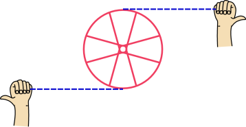 Figure 1
: Work Done on an Extended Object
- When in doubt, break the object into a large number
of small cells, and apply equation 6 to each cell
separately:
where the sum runs over all cells in the object. The idea here is
that as each cell becomes smaller, the energy associated with internal
motion within the cell becomes small ... not just small, but
disproportionately small, so that even after summing over all cells
the internal motions make a negligible contribution to the total
energy. For example, in figure 1, the center of mass of
the wheel as a whole is not moving, and the rotational kinetic energy
of the wheel is considered “internal” to the wheel. In contrast, if
we break the wheel into small cells, the center of mass of each cell
is moving, and these center-of-mass motions carry the lion’s share of
the kinetic energy. (Each cell is also rotating, but these
“internal” rotational energies are disproportionately small, and
don’t add up to much, in accordance with the scaling argument that
leads to equation 4.)
- Sometimes you can get away with using the average force and the
average displacement, if you are careful. This is important, because
the concept of work wouldn’t be practical if every time you wanted to
use it, you had to evaluate everything cell by cell, using
atomic-sized or subatomic-sized cells. It is easy to identify
two simple cases:
- As we shall see in section 4.2, if a given system or
subsystemis rigid and nonrotating, so that all parts move at the same
velocity. then it doesn’t matter where you apply the force. It is
OK to use total force and average motion.
- As we shall see in section 4.3, if the force is evenly
distributed across all the cells, in proportion to the mass of each
cell, then the internal motions of the cell don’t matter. The system
doesn’t even need to be rigid or nonrotating. You can get away with
using total force and center-of-mass velocity.
- There are undoubtedly other sufficient conditions.
We now introduce another definition of work. This definition
is somewhat more sophisticated.
Rather than talking about the work done on the object, we talk about
the work done on the boundary of the object, and more
specifically on various parts of the boundary.
For example: suppose I am pushing a car up a ramp at a steady rate. I
am pushing forward on the car, while other forces (notably a component
of the gravitational force) are pushing backwards. It certainly feels
to me like I am doing work. Indeed I am doing work, in the sense that
energy is crossing the boundary from me into the car, via the part of
the car I am pushing on. This energy flows through the car without
accumulating in the car. That is, as quickly as the energy flows into
the car (from me) it flows out again (into the gravitational field).
If we consider the car as a whole, the work is zero in this situation,
but if we divide the boundary into parts, there can be nonzero work on
this-or-that part.
3 The Work / Kinetic Energy Theorems
For each lengthscale λ, we can establish a
work[λ]/KE[λ] theorem. Specifically, for each cell, we
define work using equation 6, and the total work[λ] is
just the sum over cells in the obvious way. As we shall see in
section 7, the theorem states
We speak of the work/KE theorems, plural, because there is a separate
theorem for each lengthscale λ.
When λ is large, work[λ] is sometimes called the
pseudowork. See e.g. reference 4.
Returning to the example of pushing a car up a ramp: The KE of the car
is not changing, which is consistent with the pseudowork/KE theorem,
because the total work done on the car is zero ... even though my
local contribution to the work is nonzero.
4 Common Mode and Differential Mode
4.1 Quick Version
Another bit of terminology that may be helpful.
For any object (or cell or subcell):
This is useful because
which in turn helps you understand the
work[λ]/KE[λ] theorem.
4.2 Variations; Uniform Velocity
Starting from equation 7, we can re-express
the total work as:
where vi is the velocity of the point of application of the ith
force, i.e. the force applied to the ith cell.
Here we have written a tilde over the F~i, to remind us
that force is extensive, so that the force on an average cell is that
cell’s share of the total force. Ditto for w~i,
which represents the cell’s share of power. This stands in contrast
to the velocity, which gets no tilde because it is intensive.
We can define the average velocity as:
Similarly we can define the average share of the force:
We now define the variations:
|
δvi | | := | | vi − ⟨v⟩ |
| δF~i | | := | | F~i − ⟨F~⟩ |
| (17)
|
Hence
|
vi | | = | | δvi + ⟨v⟩ |
| F~i | | = | | δF~i + ⟨F~⟩ |
| (18)
|
and of course
Plugging equation 18 into equation 14
we find:
|
w~i | | = | | F~i · vi |
| | | = | | (⟨F~⟩ + δF~i)·
(⟨v⟩ + δvi) |
| | | = | | ⟨F~⟩·⟨v⟩
+ ⟨F~⟩·δvi
+ δF~i·⟨v⟩
+ δF~i·δvi |
| | = | | F·⟨v⟩
+ ∑ δF~i·δvi |
| (20)
|
where F is the total force (not the average share of force). Note
that the two terms that were linear in the variations dropped out,
because of the sum rule, equation 19.
The last term in equation 20 can be considered an inner
product twice over. The explicit dot product is an ordinary
three-dimensional real-space inner product ... but the sum over i
can also be considered an inner product, in an abstract
N-dimensional space. This term goes to zero if the variations in
force are perpendicular (in real space) to the variations in velocity,
in which case every term in the sum over i is separately zero
... but it also goes to zero if these terms are individually nonzero
but add up to zero, which is to say that the terms are uncorrelated.
In any case, whenever the sum over i goes to zero, it means we can
think about the system in macroscopic terms. That is, we can
calculate the work using the total force F and the average velocity
⟨v⟩.
Perhaps the simplest situation in which the sum goes to zero
is the situation where all the cells in the system
are moving with the same velocity, so that δvi = 0 for
all i.
4.3 Variations; Uniform Acceleration
We can learn something new from equation 14 if we divide
the force by mass, and multiply the velocity by mass:
|
w~i | | := | | F~i · vi |
| | | = | | (F~i / m~i) · (m~i vi) |
| | | = | | ai · p~i
|
| (21)
|
where ai is the acceleration of the ith particle, m~i
is its share of the mass, and p~i is its share of the
momentum.
The rest of the calculation runs closely parallel to
section 4.2. The only difference is that we are using
differently-weighted averages. We obtain:
where p is the total momentum of the system.
Perhaps the simplest situation in which this sum over i vanishes is
when all cells have the same acceleration, such as might result from a
uniform gravitational field. In such a case we can
multiply and divide by the total mass to obtain:
where F is the total force and vcm is the center-of-mass
velocity.
5 Remarks
- Everything in this document is restricted to nonrelativistic
mechanics only. I tried generalizing it in the
obvious way ... without success.
- Nothing we can ever do is sufficient to salvage the ghastly
“thermodynamic" formula δ E = W + Q, in which W stands for
the so-called work. As explained in reference 3, that
formula is a Bad Idea and no amount of tinkering with the definition
of W will fix it.
- This is tangentially related to the physics of friction. The
energy that is dissipated via friction is hiding in the sum over i
in equation 22: there are billions of tiny variations in
the force, slightly correlated with tiny variations in the motion.
6 Momentum
Let’s take a slight detour to talk about momentum.
Energy is important. Momentum is important. Each obeys a local
conservation law. The two concepts are intimately related, but they
are not the same.
For instance, consider a box containing 13 particles moving to the
left, plus 13 particles moving to the right, all with comparable
speeds.
|
Each of the 26 particles has some momentum, but the momentum
of the left-moving particles is opposite to the momentum of the
right-moving particles, so the system as a whole has little if any
overall momentum.
|
|
Each of the 26 particles has some kinetic energy,
and all of them make a positive contribution to the total energy of
the system.
|
|
If we apply a force to the system, it changes the momentum.
If all we care about is the momentum of the system, it doesn’t matter
where we apply the force; any force applied anywhere in the
system has the same effect on the overall momentum.
|
|
If we care about
the energy, it matters a great deal where we apply the force. A
leftward force applied to a leftward-moving particle increases the
system energy; the same force applied to a rightward-moving particle
decreases the system energy.
|
|
Specifically, the change in total momentum is:
where the index i runs over all particles in the system, pi is
the momentum of the ith particle, Fi is the force applied to that
particle, and where Ftot := ∑Fi refers to the total
force on the system.
|
|
Specifically, the change in microscopic kinetic
energy is
where xi is the position of the ith particle, and mi is its
mass. This is called the work / kinetic-energy theorem. The
notion of work is discussed in section 7; see also
reference 3.
|
|
To summarize: Momentum is denoted p and is related to
force times time.
|
|
Kinetic energy is p2/2m and is related to force
times distance.
|
7 Momentum Squared, Kinetic Energy, and Work
As discussed in section 1, we divide the system into cells.
Let’s look at the square of the momentum of one of the cells,
and see how it changes when we apply a force:
|
d (p2) | | = | | 2 p · dp |
| | | = | | 2 m v · dp |
| | | = | | 2 m v · F dt |
| | | = | | 2 m F · v dt |
| | | = | | 2 m F · dx
|
| (26)
|
or, simply,
where m is the total mass of this cell, v := p/m is the velocity
of its center of mass, x is the distance traveled by the center
of mass, and F is the total force (i.e. net force) applied to the
cell.
We rearrange it so it has dimensions of energy:
And then sum over all cells
where the sum runs over all cells.
This proves the work/KE theorem, in particular the
work[λ]/KE[λ] theorem, equation 8.
Equation 24 is useful if you know a certain force is applied
for a certain time; equation 27 is useful if you know a
certain force is applied while the cell moves a certain distance.
You might be tempted to take the limit of ultramicroscopic cells
(λ → 0). In theory, this would make the theorem
very powerful, in the sense that you would have accounted for all the
kinetic energy. In practice, the drawback is that such a theorem
would be very hard to apply, because it would require knowing every
detail of the motion and every detail of what force is applied at
which point. For example, when calculating the KE of a flywheel, do
you include the KE of electrons whizzing around inside individual
atoms? You could, but it would be unconventional and almost certainly
not worth the effort.
At the other extreme (large λ) the theorem is easy to apply,
but you have to remind yourself (and remind all other stakeholders)
that you are calculating the common-mode kinetic energy. You shouldn’t
call it “the” kinetic energy unless it is super-clear from context
that that’s what you mean.
Remarks:
- You can write the kinetic energy of any system as the
common-mode kinetic energy plus the differential-mode kinetic energy.
That is, the kinetic energy observed by Joe (in the lab frame) is
equal to the kinetic energy observed by Moe (comoving with the center
of mass) plus ½ M V2 where V is the Moe-Joe relative
velocity. This simple expression utterly depends on a special
property of the center-of-mass frame. If you have two observers
neither of which is comoving with the center of mass, the energy
transformation equations are more complicated.
- The holoscopic KE (i.e. common-mode KE) is a lower
bound on the mesoscopic KE. In turn the mesoscopic KE
is a lower bound on the microscopic KE. In general, the closer you
look, the more KE you will find.
- Given cells at a certain lengthscale, if you know the kinetic
energy of each cell separately, you can calculate the kinetic energy
at a coarser lengthscale by combining cells. But if all you know is
the total KE at one lengthscale, you can’t calculate anything but a
bound on the total KE at another lengthscale.
- The change in KE on one length scale is not a bound on the
change in KE on any other lengthscale.
- You can have a large energy transfer without a large momentum
transfer, or vice versa, as can be seen reference 5.
Here’s another interesting contrast:
|
All the forces are summed (and all the displacements are
summed) before multiplying.
The sum over displacements is a
weighted sum, weighted by mass.
|
|
Each microscopic force is multiplied by the corresponding
microscopic displacement before summing.
|
In general, it makes a huuuuge difference whether the multiplication
occurs before or after the summation. It also makes a huuuuge
difference whether or not a weighted sum is used.
8 References
-
-
John Denker,
“Welcome to Spacetime”
www.av8n.com/physics/spacetime-welcome.htm -
John Denker,
“Spacetime Kinetic Energy – An Exercise in Numerical Methods”
www.av8n.com/physics/spacetime-kinetic-energy.htm -
John Denker,
“Work” (chapter in Modern Thermodynamics)
./thermo-laws.htm#sec-def-work -
B. A. Sherwood and W. H. Bernard,
“Work and heat transfer in the presence of sliding friction”
Am. J. Phys 52(11) (1984).
http://www4.ncsu.edu/~basherwo/docs/Friction1984.pdf -
John Denker,
“What Makes the Car Go”
./car-go.htm