Single- and Multi-Variable Linear Least Squares
John Denker
1 Introduction
Linear least squares is also known as linear regression. It is used
for fitting a theoretical curve (aka model curve, aka fitted function)
to a set of data.
Fun fact #1: The word “linear” in this context does mean that the
fitted function is a straight line (although it could be). It could
perfectly well be a polynomial, where the monomials are nonlinear, or
it could be a Fourier series or some such, where the basis functions
are highly nonlinear. The key requirement is that the
coefficients i.e. the parameters that you are adjusting
must enter the fitted function linearly.
Linear regression is by no means the most general or most
sophisticated type of data analysis, but it is widely used because it
is easy to understand and easy to carry out.
* Contents
2 A Simple Example : Determining Density
Let’s start with a simple example. (A less-simple more-realistic
example is discussed in section 4. Some of the
principles involved, and some additional examples, are presented in
section 5.)
Suppose we want to compute the density of some material, based on
measuring three samples. The volume and mass of the samples are shown
in table 1.
| V | | M |
| Volume | | Mass |
| 1.000 | | 1.062 |
| 1.100 | | 1.091 |
| 1.200 | | 1.211 |
Table 1: Volume and Mass – Raw Data
This is Monte Carlo data, which is a fancy way of saying it was cooked
up with the help of the random-number generator on a computer. The
volume readings are evenly spaced. The mass readings are drawn from a
random distribution, based on a density of ρ=1 (exactly) plus
Gaussian random noise with a standard deviation of 0.05. All the
data and plots in this section were prepared using the spreadsheet in
reference 1.
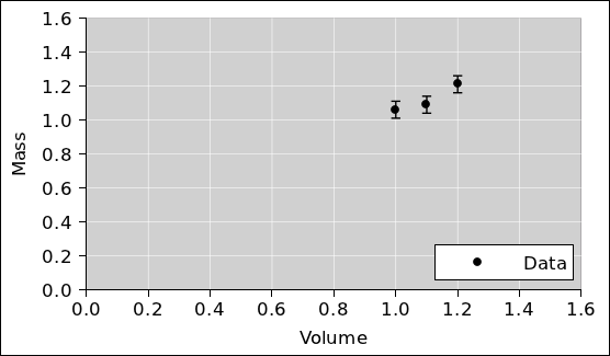
- 1.
In accordance with standard good practice, the first
thing to do is to plot the data and look at it, to see whether it
makes sense. This is shown in figure 1. When we
look at this, nothing jumps out at us, which is OK.
- 2.
The obvious next step is to calculate the density.
We do this for each sample, on a sample-by-sample basis, as shown in
table 2.
| V | | M | | ρ |
| Volume | | Mass | | Density |
| 1.000 | | 1.062 | | 1.062 |
| 1.100 | | 1.091 | | 0.992 |
| 1.200 | | 1.211 | | 1.010 |
| | |
| | | | | Naïve |
| | | | | Average |
| | | | | 1.021 |
Table 2: Volume, Mass, and Calculated Density
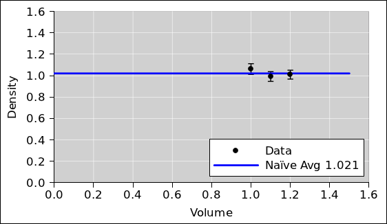
We plot this data as well, and look at it.
We can estimate the average density graphically, by hand, with the
help of a transparent ruler. Draw a horizontal line so that the data
points are distributed symmetrically above and below the line.
Note:
- It is important that the ruler be transparent. Otherwise
you will introduce bias, typically by under-emphasizing the data
points that are not visible.
- It is important to keep the line horizontal. Zero slope.
This is easier to do if you plot the data on graph paper (as opposed
to unadorned typing paper).
Optionally, we can take the average of these three densities
numerically, as shown at the bottom of table 2,
although this is slightly naïve (for reasons discussed in
item 3). The value we compute is very nearly the same as
the value corresponding to the height of the horizontal line we drew
using the transparent ruler, which makes sense. This is plotted in
figure 2.
Note that taking the average is tantamount to a one-parameter fit.
There is only one quantity to be determined from the data, namely the
average density.
- 3.
We can perform a less-naïve analysis if we realize
that the mass data has uniform error bars but the density data does
not. That’s because when we divide the mass by the volume, the error
bars get divided also. Therefore we should perform a weighted
average, giving the larger samples larger emphasis, in proportion to
the inverse square of the error bars.
| V | | M | | ρ | | Weight | |
| Volume | | Mass | | Density | | Factor | |
| 1.000 | | 1.062 ±.05 | | 1.062 ±.05 | | 1.000 | |
| 1.100 | | 1.091 ±.05 | | 0.992 ±.046 | | 1.210 | |
| 1.200 | | 1.211 ±.05 | | 1.010 ±.042 | | 1.440 | |
| | |
| | | | | Naïve | | Weighted | |
| | | | | Average | | Average | |
| | | | | 1.021 | | 1.018
| |
Table 3: Volume, Mass, and Weighted-Average Density
Again, we plot the data and look at it. Again we note that taking the
average is tantamount to fitting the data using a one-parameter model
i.e. a zeroth-order polynomial i.e. a horizontal straight line.
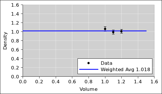 Figure 3
: Density Data plus Weighted Average
- 4.
It is possible to analyze the raw
mass-versus-volume data directly, using it in the form we see in
figure 1, without explicitly calculating the density
of each sample. This is a tricky approach. It works fine if done
properly, but we have to be careful.
The key step in the analysis is to draw a straight line through the
data, as shown in figure 4.
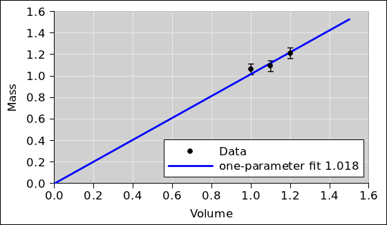 Figure 4
: Mass versus Volume plus Fitted Line
This can be done by hand using a transparent ruler. Draw a line so
that the data points are distributed symmetrically above and below the
line. Note:
- As mentioned in item 2,
it is important that the ruler be
transparent.
- It is important to pin the ruler so that the fitted line goes
through the origin. We know for sure that the graph of mass versus
density must do this, in accordance with equation 1b.
We know this absolutely, a priori, as a consequence of the
official definition of density, equation 1a.
|
ρ | | := | | M / V | |
(1a)
|
| M | | = | | ρ V | |
(1b)
|
|
Pinning the ruler gives us a one-parameter model. In fact if we do it
properly, it gives the same result as the weighted average in
item 3 – the same conceptually, numerically, and in every
other way. It should come as no surprise that we want a one-parameter
model, given that we used one-parameter models in item 2
and item 3. See section 3.1 for more about how and
why we pin the ruler.
Refer to section 3.2 and section 3.3, if you dare,
for a discussion of some of the misconceptions that can arise in
conjunction with this approach.
- 5.
We can also use a computer to calculate the best-fit
straight line directly. Specifically, we can use the
linest(y_vec, basis_vecs) spreadsheet function. The result
is identical to what we see in figure 4. The
slope found by linest(...) is exactly equal to the
weighted-average density we calculated in
table 3, as it should be.
- 6.
When using a computer – just as when using a transparent ruler
– it is important to constrain the fit so that the mass-versus-volume
curve goes through the
origin. This can be arranged by setting to zero the optional third
argument to the linest(...) function. Keep in mind that
equation 1b is of the form y=mx which has one adjustable
parameter (the slope). It is emphatically not of the form y=mx+b
which would have two adjustable parameters (the slope and the
y-intercept). When linest(...) peforms the fit, we need it to
perform a one-parameter fit, not a two-parameter fit.
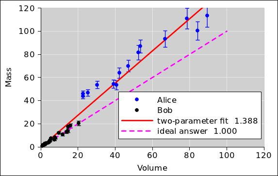
If you don’t believe me, take a look at
figure 5. The red line shows what would
happen if you performed a two-parameter straight-line fit. It’s a
horror show. The slope of the two-parameter fit is wildly different
from the actual density. The one-parameter fit (shown in blue) does a
much, much better job.
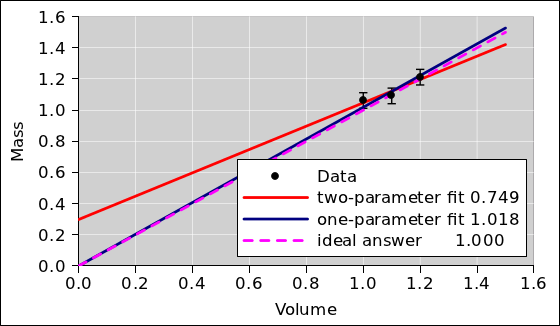 Figure 5
: One-Parameter versus Two-Parameter Fit
Keep in mind that the details depend on how much data we have, and now
noisy it is. If we had 300 data points rather than 3 data points, we
would be better able to afford adding fitting parameter, but even then
we would need some specific rationale for doing so.
3 Discussion
3.1 How and Why We Pin the Ruler
In connection with figure 5, when we speak
of pinning the ruler, you could use an actual push-pin (with a
suitable backing pad), but the usual good practice is to use your
pencil or pen. Hold the tip of your pen at (0, 0). Gently push the
ruler up against it, and use it as a pivot. In other words, use your
pen as a pin. This trick is widely used by artists, wood-shop and
metal-shop workers, draftsmen, et cetera.
Note that the situation shown in figure 5
is very common and utterly typical. The red line illustrates an
important general principle, namely that it is a very bad idea to use
“extra” adjustable parameters when fitting your data. This
principle is known as Occam’s Razor and has been known for more than
700 years.1 Narrowly speaking, the red line does a better of
fitting the data; it just does a much worse job of
explaining and modeling the data. That is to say, the red
line actually comes closer to the data points than the blue line does.
However, our goal is to interpret the data in terms of density, and
the red line does not help us with that. Equation 1b
provides us with a sensible model of the situation, and the blue line
implements this model. The slope of the blue line can be directly
interpreted as density.
Some descriptive terminology:
- In the statistics literature, this situation is sometimes
referred to as a bias-variance tradeoff.
- If you use too many parameters, you wind up fitting the
noise (rather than fitting the signal).
- Similarly, using too many parameters is known as
overfitting the data.
For a simple yet modern introduction to the fundamental
issues involved, see reference 2.
See section 3.3 for more about the
perils of superfluous parameters.
If not pinned, the ruler implements at two-parameter model. Just
because you could use a two-parameter model doesn’t mean you
should. Just because the tool allows a two-parameter fit doesn’t mean
it is a good idea. As the ancient proverb says,:
It is a poor workman
who blames his tools.
|
|
|
|
3.2 How Not to Pin the Ruler
This section exists only to deal with a misconception. If you don’t
suffer from this particular misconception, you are encouraged to skip
this section.
Some people try to explain pinning the ruler by saying we are fitting
the curve to an imaginary data point at (0, 0) ... but I do not
recommend this way of thinking about it. It is better to base
the decision on good, solid theory than on imaginary data. We
do indeed have a good, solid theory, namely the definition of
density, equation 1a.
In some sense it would be the easiest thing in the world to take data
at (0, 0). We know exactly how much a zero-sized sample weighs, and
we know exactly how much volume a zero-sized sample displaces. So
this data point is in some sense more accurate than any of the data
you see in table 3. However, this data
point would be hard to analyze using the method of
table 3, because we cannot divide zero
mass by zero volume to get information about the density. This is
harmless but uninformative. It just reflects the fact that for any
density whatsoever, the mass-versus-volume curve must pass through
(0, 0).
It must be emphasized that all the calculations involved in
table 3 can be and should be done
without reference to any imaginary data at the origin ... or any real
data at the origin. In third grade you learned how to divide one
number by another, and that is all that is needed to calculate the
density in accordance with equation 1a.
Starting from
you can, if you want, rewrite this so that it looks like the slope of
a line:
|
ρ | | = | | | |
(3a)
|
| | | = | | | |
(3b)
|
| | | = | | slope from (0,0) to (V,M) ??? | |
(3c)
|
|
You are free to do this, but you are not required to. Furthermore,
the legitimacy of the step from equation 2 to
equation 3a is guaranteed by the axioms of arithmetic. It
does not depend on any fake data (or real data) at the origin.
Let’s be clear: I do not want to hear any complaints about “fake”
data at the origin, for multiple reasons:
- There is no need to use any data at the origin, fake or
otherwise. There is no need to even mention the origin. You
learned in third grade how to divide one number by another, and that
is all that is required. You are not obliged to interpret the
density in terms of the slope of a line. If you want to make this
dubious interpretation as shown in equation 3c, do so at
your own risk.
- Consider the fitting procedure: Data goes in, and a fitted
model comes out. No matter whether or not you use any (0, 0) data
as input, the fitted mass-versus-volume curve that comes out will
pass through the origin, assuming we do things properly. This is
guaranteed by the definition of density.
- If you wanted to take some non-fake data at the origin,
or infinitesimally close to the origin, you could do so.
- If you create an artificial problem, you ought not brag if you
manage to solve it. If you create an unnecessary problem, you ought
not whine if you fail to solve it. Using a two-parameter model of
the form y=mx+b for the density is an artificial, unnecessary
problem of just this sort. You can partially alleviate or conceal
the damage by using fake data (or real data) at or near the origin
to constrain the extra parameter at the only reasonable value,
namely b=0. You ought not brag about or whine about this partial
success. The fundamental point is that you should have been using a
one-parameter model all along.
The whole idea of using a two-parameter model in mass-versus-volume
space is sophomoric, i.e. pseudo-sophisticated yet dumb at the same
time. The normal approach would be to calculate the densities and
then average them in the obvious way, as in
figure 3. People get into trouble if they are
sophisticated enough to realize that they can analyze the data in
mass-versus-volume space, but not sophisticated enough to do it
correctly.
3.3 How Not to Justify Superfluous Parameters
This is another section that exists only to deal with a misconception.
If you don’t suffer from this particular misconception, you are
encouraged to skip this section.
Sometimes people who ought to know better suggest that “extra”
parameters are a way of detecting and/or dealing with systematic
errors. This is completely wrong, for multiple reasons.
Example #1: Let’s consider the scenario where Alice and Bob
are lab partners. Alice takes some of the data, and Bob takes the
rest. Alice screws up the tare, but Bob doesn’t. The data is shown
in figure 6. Specifically, the
two-parameter straight-line fit to the data, as shown by the red line,
has a negligible y-intercept. The slope, meanwhile, is
significantly wrong i.e. not equal to the actual density.
It should be obvious that in this scenario, allowing for a nonzero
y-intercept is nowhere near sufficient to detect the problem, let
alone resolve it.
In contrast, plotting the data and looking at it, as suggested in
item 1, helps a lot.
To repeat: You should never increase the number of parameters in your
model without a good reason. Mumbling vague words about some
unexplained “experimental error” is never a sufficient rationale.
That’s the sort of thing that leads to the disaster shown by the red
curve in figure 5 and/or
figure 6.
Example #2: If you systematically use the wrong units,
e.g. CGS units (g/cc) instead of SI units (kg/m3), there
result will suffer from a huge systematic error, but fitting
the data using a superfluous y-intercept will be completely
ineffective at detecting the problem, let alone resolving it.
Example #3: Porosity can cause systematic errors in any
determination of density. These cannot be reliably detected, let
alone corrected, by throwing in an “extra” parameter without
understanding what’s going on. See section 4.
Example #4: If you forgot to tare the balance in a way that
affected all the data equally, it would lead to a nonzero
y-intercept on the pseudo-mass-versus-volume curve. However, the
converse is not true. The huge y-intercept on the red curve in
figure 5 is absolutely not evidence of a
screwed-up tare. Conversely, the absence of a significant
y-intercept in figure 6 is absolutely not
evidence of the absence of systematic error. Furthermore, even if the
data behind figure 5 included a screwed-up
tare, using a two-parameter fit would not be an appropriate way to
resolve the problem. It would just add to your problems. You would
have all the problems associated with the red curve in
figure 5, plus a screwed-up tare. The
correct procedure would be to go back and determine the tare by direct
measurement. If this requires retaking all three data points, so be
it.
The red curve in figure 6 shows what
happens if you try to detect and/or deal with a problem without fully
understanding it. Again, the best procedure is to do things right the
first time. In an emergency, if you wanted to correct the mistake in
figure 6, you would first need to
understand the nature of the mistake, and then cobble up a complicated
model to account for it. Just throwing in an adjustable y-intercept
and hoping for the best is somewhere between unprofessional and
completely insane.
If you have a very specific, well-understood nonideality in your
experiment, the best procedure is to redesign the experiment to remove
the nonideality. The second choice would be to make a richer set of
measurements, so that you get independent observations of whatever is
causing the nonideality ... for instance by making independent
observations of the tare. Failing that, if you are sure you
understand the nonideality, it might be OK to complexify the model so
that it accounts for that specific nonideality, such as the fancy
stepwise correction we see in the cyan curve in
figure 7. We use a model of the form
y=mx for Bob’s data and a model of the form y=mx+b for Alice’s
data. Note that m is the same for both, as it should be, since we
are trying to determine the density and it should be the same for
both. In this scenario we have an order of magnitude more data than
we did in section 2 41 points instead of 3 points – so
the additional parameter (b) does not cause nearly so much
trouble. Away from the step, the slope (m) of the cyan curve is
constant and is a very good estimate of the density we are trying to
measure. However, even in the best of circumstances, adding variables
comes at a cost. You need to make sure you have enough data points
(and short enough error bars) so that you can successfully ascertain
values for all the parameters. That is, you need to make sure you are
on the right side of the bias/variance tradeoff.
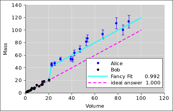 Figure 7
: Fancy Correction for Well-Understood Error
3.4 Maximum Likelihood, Or Not
Keep in mind that all the methods discussed in this document are
least-squares methods. That means they are in the category of
maximum likelihood methods. In other words, they calculate the
conditional probability of the data, given the model. For virtually
all data-analysis purposes, that’s the wrong way around. What you
really want is the probability of the model, given the data. The
details of how to do this right are beyond the scope of this document.
For simple tasks such as the density determination in
section 2 you can get away with maximum likelihood, but
please do not imagine that there is any 11th commandment that says
maximum likelihood is the right thing to do. A lot of people who
ought to know better assume it is OK, even when it isn’t.
3.5 Data Analysis : Closing the Loop
Whenever you need to analyze data, you should test your methods. The
procedure outlined in section 2 is a good empirical check
(but not the only possible check).
Starting from a set of reasonable parameters, generate some artificial
data. Add some Monte Carlo noise to the data. Then analyze the data
and see how accurately you get the right answer, i.e. how closely the
fitted parameters agree with the parameters you started with.
This kind of check is called “closing the loop” around the data reduction
process. The closed loop is shown in figure 8.
Closing the loop is considered standard good practice aka due diligence.
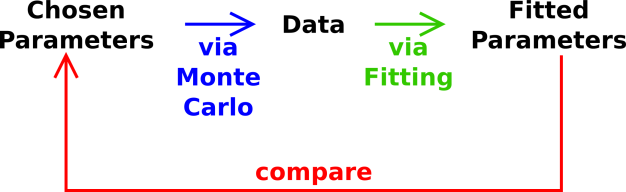 Figure 8
: Closing the Loop around the Analysis
3.6 More General Regression Curves
The linest(...) spreadsheet function is often used for finding
a “trend line” ... but it is capable of doing much more than
that. In general, it finds a regression curve,
which not be a straight line.
- It can find the coefficients of the best-fit quadratic.
An example of this is given in section 5.7.
- It can also handle higher-order polynomials.
- It can find the coefficients of the best-fit Fourier
series. An example of this is given in section 5.8.
- More generally, it can fit to an arbitrary linear combination
of basis functions, using whatever basis functions you choose.
In statistics, this fitting procedure is called linear
regression. It must be emphasized that this method requires the
fitted function (the regression curve) be a linear combination of the
basis functions, but the basis functions themselves do not need to be
linear functions of X (whatever X may be).
4 Density, Again
Let’s do another density determination. This time the task will be
somewhat more realistic and more challenging. We will have to apply a
higher degree of professionalism. The spreadsheet used to construct
the model and do the analysis is available; see
reference 1.
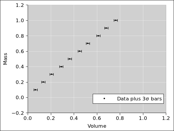
In the real world, it is usually easier to measure mass accurately
than to measure volume accurately. Therefore, in this section we have
arranged for the artificial data to have significant error bars in the
volume direction but not in the mass direction, as you can see in
figure 9.
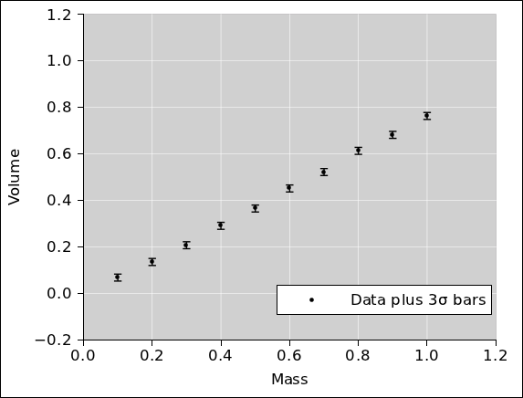
In a logical world, data-analysis procedures would be able to handle
uncertain abscissas just as easily as uncertain ordinates. However,
the most commoly-available procedures are not as logical as you might
have hoped. They do not handle uncertain abscissas at all well.
Therefore in figure 10 we replot the data using
mass as the abscissa. It must be emphasized that
figure 9 and figure 10
are two ways of representing exactly the same data. (For clarity, the
error bars in these two figures are 3σ long. All other figures
use ordinary 1σ bars.)
We divide mass by volume to get the density. This is done
numerically, on a sample-by-sample basis, just as we did in
section 2. The numerical data table can be found in
reference 1. The results are plotted in
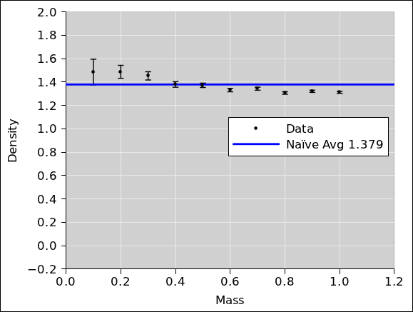
figure 11. The naïve (unweighted) average
is also shown.
At first glance, the data doesn’t look too terrible. However, if you
look more closely, it looks like there might be something fishy going
on. The low-mass data might be systematically high, while the
high-mass data might be systematically low.
It’s hard to tell what’s going on just by looking at the data in this
way. The professional approach is to look at the residuals. That is,
we subtract the fitted average from the data and see what’s left.
Even better, if possible, we normalize each of the residuals by its
own error bar. Then, to make the data fit nicely on the graph, we
reduce the residuals by a factor of 10. This is shown in
figure 12. The properly-weighted
average is also shown.
Note that normalizing the residuals is easy for
artificial data but may be more difficult for real-world data. At
this stage in the analysis, you might or might not have a good
estimate for the error bars on the data. If necessary, make an
order-of-magnitude guess and then forge ahead with the preliminary
analysis. With any luck, you can use the results of the preliminary
analysis to obtain a reasonable estimate of the uncertainy. You can
then re-do the analysis using the estimated uncertainty, and check to
see whether everything is consistent.By the same token, it is pointless to quote the chi-square of a fit,
if you are depending on the fit to obtain an estimate of the
uncertainty of the data.
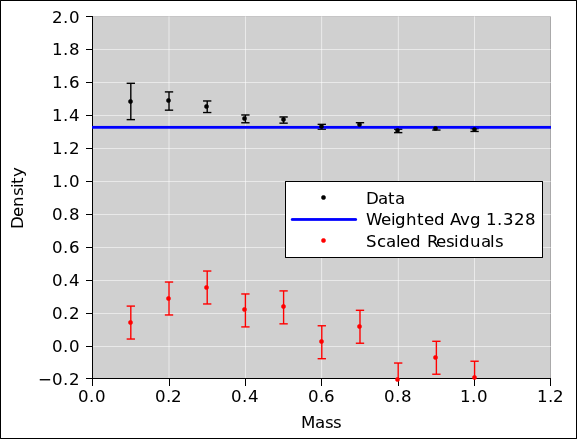 Figure 12
: Density versus Mass, with Residuals
Our suspicions are confirmed; there is a definite northwest/southeast
trend to the residuals. This is not good. There is some kind of
systematic problem.
As mentioned in section 3.3, sometimes people who ought to
know better suggest that throwing in a superfluous fitting parameter
is a good way to check for and/or correct for systematic errors.
Applying this idea to our example gives the results shown in
figure 13. As you can see, adding a parameter
to the model without understanding the problem is somewhere
between unprofessional and completely insane. It is not successful in
detecting (let alone correcting) the problem.
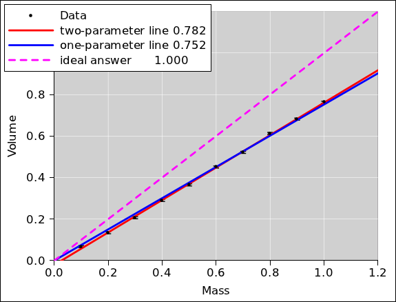 Figure 13
: Volume versus Mass, Fit with “Extra” Parameter
After thinking about the problem for a long time, we discover that the
material is slightly porous. When we measure the volume by seeing how
much water is displaced by the sample, the water percolates into the
sample for a distance of 0.2 units. As a result, there is a “shell”
surrounding a “core”. Specifically, it turns out that all along,
the data was synthesized by stipulating that the effective
displacement of the sample is 100% of the core volume plus 2/3rds of
the shell volume, plus some noise.
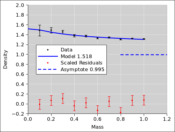
Now that we understand what is going on, we can build a
well-founded model. Specifically, we will fit to a two-parameter
model, hoping to find the density of the core and the (apparent)
density of the shell. The results are shown in
figure 14.
Note that the residuals are much better behaved now. They
are closer to zero, and exhibit no particular trend.
As you can see from the y-intercept of the model, the apparent
density of the shell is 1.518. This is very nearly the ideal answer
i.e. 1.5 i.e. the reciprocal of 2/3rds.2
Meanwhile, the other fitted parameter tells us the asymptotic density,
i.e. the density of the core, which is 0.995. This is very nearly the
ideal answer i.e. 1.0. Note that this is incomparably more accurate
than the result we would have gotten via simple one-parameter
averaging (as in figure 12) or via a
dumb two-parameter straight-line fit (as in
figure 13). Even if you took data all the way
out to volume=10 or volume=100 the shell would cause a significant
systematic error. That is to say, the apparent density of the sample
approaches the asymptotic density only slowly ... very very slowly.
You can see that in order to make an accurate determination of the
density of the material, it was necessary to account for the
systematic error. Random noise on the mass and volume measurements
was nowhere near being the dominant contribution to the overall error.
- In this example, we chose to deal with the systematic error by
building a model that accounts for what is going on. This is a tricky
business, building something that is detailed enough to be a faithful
model, yet not so complicated that it introduces too many additional
adjustable parameters.
- Another approach would be to change the experimental method so
that it is less sensitive to porosity. One could imagine using 3D
laser scanning (rather than liquid displacement) to ascertain the
volume. Alternatively, depending on the material, one could imagine
sculpting it into an accurate spherical shape, measuring the diameter
with calipers, and using that to infer the volume.
If the data had been less noisy, the importance of dealing with the
systematic error would have been even more spectacular. (I dialed up
the noise on the raw data to make the error bars in
figure 9 more easily visible. The downside is
that as a result, the systematic errors are only moderately
spectacular. They don’t stand out from the noise by as many orders of
magnitude as they otherwise would. It is instructive to reduce the
noise and re-run the simulation.)
5 Principles of Linear Least-Squares Fitting
5.1 Basic Notions
In general, linear regression can be understood as follows. We want
to find a fitted function that is a linear combination of certain
basis functions.
To say the same thing in mathematical terms, we want to find a
best-fit function B that takes the following form:
|
| |
B(i) | | = | | a0 b0(i)
+ a1 b1(i)
+ a2 b2(i)
+ ⋯
+ aM−1 bM−1(i) | |
(4a)
|
|
| |
| | = | | | |
(4b)
|
|
The aj are called the coefficients, and the bj are called the
basis functions. There are M coefficients, where M can be any
integer from 1 on up. Naturally, there are also M basis
functions.
Using vector notation, we can rewrite equation 4 as
|
| |
B(i) | | = | | a · b(i) | |
(5a)
|
|
| |
| | = | | ⟨a | b(i)⟩ | |
(5b)
|
|
where a is an M-dimensional vector, and where b is a
vector-valued function of i. Equation 5b uses Dirac
bra-ket notation to represent the dot product.
Given a set of observed Y-values {Y(i)} and a set of basis
functions, the simplified fitting procedure finds the optimal
coefficient-vector ⟨a| ... where “optimal” is defined in
terms of minimizing the distance
where Du is the naïve unweighted distance. The weighted distance
is:
When minimizing D, you can ignore the denominator in equation 7, since it is a constant.
It must be emphasized that the coefficients aj are always
independent of i; that is, independent of which data point we are
talking about. In contrast, the weights wi depend on i but are
independent of j, i.e. independent of which basis function we are
talking about.
5.2 Weighting
Pedagogical suggestion:
- When first introducing the topic, don’t even mention weights.
Let all fits be unweighted, by which we mean equally-weighted.
This applies to curve fitting in general, and to averaging in
particular, which I consider to be just a particularly simple type
of curve fitting.
- On the next turn of the pedagogical spiral, the motto
should be:
-
All averages are weighted averages.
- All fits are weighted fits.
In this section, we assume each data point has a nontrivial
weight associated with it. If the data is uncorrelated, we
should minimize the weighted distance:
where σ(i) is the uncertainty on the ith point, and the
weighting factor W(i) ≡ 1/σ2(i) tells how much emphasis
to give the ith point. Alas the spreadsheet linest(...)
function does not allow you to specify the weights. It forces you to
give all the points the same weight. This is, in general, a very bad
practice. The workaround for this problem is to pull a factor of
σ(i) out of every point in the data, and out of every point in
every basis function. This is doable, but incredibly annoying. Among
other things, it means the supposedly-constant function b0(i) in
equation 11a is no longer constant, i.e. no longer independent of
i. This means you must set the third argument of
linest(y_vec, basis_vecs, affine) to zero, and then supply
your own b0(i) function as one of the basis functions in the second
argument.
More generally, we can handle correlated raw data as follows:
|
D | | = | | | [Y(i) − a · b(i)]
wij
[Y(j) − a · b(j)]
|
|
| (9)
|
where w is the weight matrix.
Typical spreadsheet programs have a linest() function that
doesn’t know anything about weights. For uncorrelated data, you can
compensate for this easily enough, as follows: For each data point
i, multiply the observed Y(i) and each of the basis functions
b(i) by 1/σ. This produces the required factor of
1/σ2 in the objective function, in accordance with equation 8.
This is of course synonymous with multiplying the data and the
objective functions by √(wii), in accordance with
equation 9.
In the linest() function, you not enable the built-in
feature that gives you a constant term. You need a column of
constants to which weighting can be applied. Other than that, you do
not need to allocate any new rows or columns, because you can do the
division on the fly, dividing one array by another. If the
observations are in column Y, the basic functions are in columns
ABC, and the weights are in column W, you can use an expression
like this:
=linest(Y1:Y10/W1:W10, A1:C10/W1:W10, 0, 1)
An example of this can be found on one of the sheets in reference 3.
5.3 Often, The Weights Come From the Model
Consider the data shown in figure 15.
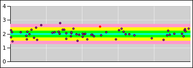 Figure 15
: Randomness = Property of the Distribution
You will notice that the data points to not have
error bars associated with them.
Instead I used the model to plot:
- a best-fit line (the central cyan line)
- a 1σ tolerance band (the green shaded region)
- a 2σ tolerance band (the yellow shaded region)
- a 3σ tolerance band (the pink shaded region)
The model (including the tolerance band) is plotted in the background,
and then the zero-sized pointlike data points are plotted in the
foreground.
I am not the only person to do things this way. You can look at
some data from the search for the Higgs boson. The slide shows the
1σ (green) and 2σ (yellow) bands. The data points are
pointlike. We get to ask whether the points are outside the band.
Reference 4 intro goes into more detail on this
point, and shows additional ways way of visualizing the concept.
Search for where it talks about “misbegotten error bars”. The
point is, putting error bars on the raw data points is just wrong. It
will give you the wrong fitted parameters. I am quite aware that
typical data-analysis texts tell you to do it the wrong way.
Now the question arises, how do we achieve the desired state. In
favorable cases, the weights can be determined directly from the
abscissas. In least-squares fitting, the abscissas are considered
known, so determining the weights is straightforward.
Sometimes, however, the weights depend on the model in more
complicated ways. They may depend on the fitted parameters. This is a
a chicken-and-egg problem, because the fitting procedure requires
weights in order to do the fit, yet the fitted parameters are needed
in order to calculate the weights.
The solution is to pick some initial estimate for the weights, and do
an initial fit. The use the fitted parameters to obtain better
weights, and iterate.
Let’s apply this to the example in reference 3.
In order of decreasing desirability:
- You could measure the weight of the spring, and use theory to
set the initial extra-mass parameter to 1/3rd of the mass of the
spring. This is exact for an ideal spring. It is only approximate
for real springs, but it’s good enough for an initial estimate.
- You could set the extra-mass parameter to zero, as a first
approximation. The weights then depend only on the bob mass,
which is known in advance.
- If you’re really lazy, you could use uniform weights as
an initial guess.
Note that nonlinear least-squares fitting is always iterative. If you
have to hunt for suitable weights, even linear least-squares fitting
becomes iterative.
5.4 Background: What’s Linear and What’s Not
The documentation for linest(...) is confusing in at least two
ways:
The documentation claims the linest() function explains Y(i)
in terms of what it calls “X(i)” but we are calling the basis
functions bj(i). We write “X(i)” in scare quotes to avoid
confusion. In fact, in terms of dimensional analysis, the basis
functions don’t even have the same dimensions as x. Consider the
case where y(x) is voltage as a function of time; the basis
functions necessarily have dimensions of voltage, i.e. the same as y
(not time, i.e. not the same as x). IMHO the linest()
function should be documented as linest(y_vec, basis_vecs,
...) or something like that.
In contrast, the genuine x (without scare quotes) means something
else entirely: Suppose you think of y as a function of genuine x,
plotted on a graph with a y-axis and a x-axis. Then it is
emphatically not necessary for this genuine x to be one of the basis
functions bj. The poster child for this is a Fourier series (with
no DC term), where the genuine x is not one of the basis functions.
Let’s be clear: the fitting procedure cares only about bj(i), that
is, the value of the jth basis function associated with the ith
data point. It does not care about the genuine x-value associated
with the ith point, unless you choose to make x one of
the basis functions. The x-axis need not even exist.
To say the same thing another way: Linear regression means that the
best-fit function B needs to be a linear function of the parameters
aj. It does not mean that the jth basis function bj(i) needs
to be a linear function of i. Again, the poster child for this is a
Fourier series (with no DC term), where none of the basis functions is
linear. |
Here’s another point of possible confusion:
The documentation says you should set the third argument (affine)
to TRUE if «the model contains a constant term». What
it actually means is that third argument should be set to TRUE
if (and only if) you want an x0 basis function to be thrown into the
model in addition to whatever basis functions you specified
explicitly in the second argument.
To say the same thing the other way, if you included an explicit
x0 basis function in the second argument, the third argument
needs to be FALSE.
In particular, if you are doing a weighted fit (as you almost
certainly should be), you need to set the third argument
(“affine”) to FALSE and provide your own x0 points,
properly weighted. (There is no way to apply weights to the
built-in “affine” term.) |
5.5 Example: Fitting a Straight Line
Keep in mind the warning in section 5.4: The basis
functions do not need to be linear. A lot of people are confused
about this point, because the special case described by
equation 11 is the most common case. That is to say, it is
common to choose the genuine x-value to be one of the basis
functions. Not necessary but common. We can express that
mathematically as:
|
b1(i) | | = | | I(x(i)) | | (the identity function) |
| | | = | | x(i) | | (for all i) |
| (10)
|
where x(i) is the genuine x-value that you plot on the x-axis.
In particular, fitting a straight line with a two-parameter fit means
choosing b1 to be the identity function (equation 10 or
equation 11b), and choosing b0 to be the trivial constant
function (equation 11a):
|
b0(i) | | = | | 1 | | (for all i) | |
(11a)
|
| b1(i) | | = | | x(i) | | (for all i) | |
(11b)
|
|
This linear equation can be contrasted with the quadratic in
equation 14.
A one-parameter fit is used when the straight line is constrained to
go through the origin. It omits the constant basis function
(equation 11a).
5.5.1 Fitting to Points Within an Error Band
Figure 16 shows a straight line fitted to four data points.
Because of the symmetry of the situation, the fitted line has zero slope.
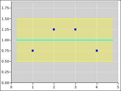 Figure 16
: Straight Line Fitted to 4 Points; Equally Weighted
Figure 17 shows the same situation, except that
it is a weighted fit. Point #3 has four times the weight of any of
the other points. The weight comes from the model. The model says
that the error band is only half as wide at abscissa #3.
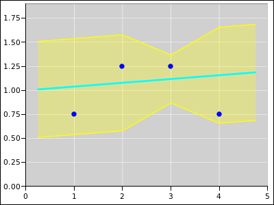 Figure 17
: Straight Line Fitted to 4 Points; Extra Weight on Point #3
Figure 18 shows the same situation, except that
oint #4 is the one with the extra weight.
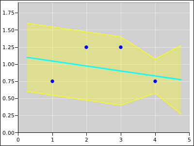 Figure 18
: Straight Line Fitted to 4 Points; Extra Weight on Point #4
5.5.2 Fitting to Distributions with Error Bars
A lot of people are accustomed to thinking in terms of error bars.
This is very often the wrong thing to do. When fitting to raw data
points, such as the blue points in section 5.5.1, it is
better to think in terms of zero-sized pointlike points, with no error
bars, sitting within an error band.
However, sometimes you get information that is not in the form of raw
data points, but rather cooked distributions. The width of the
distribution can be represented by error bars. Let’s be clear: the
blue plotting symbols in section 5.5.1 represent numbers,
whereas the red plotting symbols in this section represent
distributions. A number is different from a distribution as surely as
a scalar is different from a high-dimensional vector.
The mathematics of weighted fitting is the same in this case, even
though the interpretation of resulting fit is quite different. This
is shown in the following diagrams.
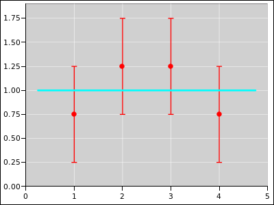 Figure 19
: Straight Line Fitted to 4 Distributions; Equally Weighted
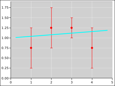 Figure 20
: Straight Line Fitted to 4 Distributions; Extra Weight on #3
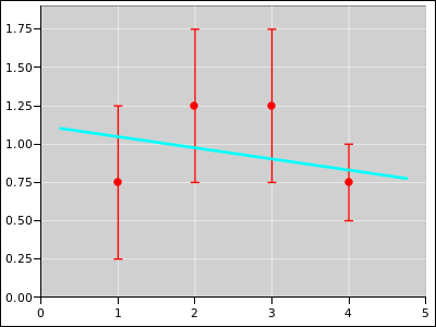 Figure 21
: Straight Line Fitted to 4 Distributions; Extra Weight on #4
5.6 Tactics: Weighted Linest
It is not difficult to perform weighted fits using the usual
implementation of linest(), even though the documentation
doesn’t say anything about it. The procedure is messy and arcane, but
not difficult.
The first step is to not use the built-in “affine” feature.
Instead create an explicit basis function with constant values,
as in equation 11a. This basis function can be weighted,
whereas the built-in “affine” feature cannot.
The next step is to create a copy of all your y-values and all your
basis functions, scaled by the square root of the weight:
|
y′(i) | | = | | |
|
b′j(i) | | = | | | for all j |
| (12)
|
Then apply the linest() function to the primed quantities.
Note that the weight of a point is inversely proportional to the
uncertainty squared. So multiplying by the square root of the
weight is the same as dividing by the uncertainty to the first power:
|
y′(i) | | = | | y(i) / σ(i) |
|
b′j(i) | | = | | bj(i) / σ(i) | for all j |
| (13)
|
The scaling factor applied by these equations affects both terms
within the square brackets in equation 6b. It
gets squared along with everything else, so the effect is the same as
the weighting factor in the numerator of equation 7, as desired.
Keep in mind that linest() has no notion of continuity of y
as a function of x. It treats the ith point (xi, yi)
independently of all other points. Therefore scaling the y-values
in accordance with equation 12 does no harm. It has no
effect other than the desired weighting factor.
Summary:
Divide by the error bar, or equivalently
multiply by the square root of the weight.
|
|
|
|
5.7 Another Example: Fitting a Quadratic
A quadratic is perhaps the simplest possible nonlinear function.
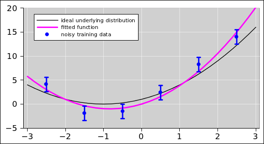
Figure 22 shows an example of using multi-parameter
least-squares fitting to fit a quadratic to data. The fit (and the
figure) were produced using the "polynomial-plain" page of the
spreadsheet in reference 5.
In the figure, the blue points are the observed data. For the
purposes of this example, the data was cobbled up using the ideal
distribution given by the black curve, plus some noise. (In the real
world, you do not normally have the ideal distribution available; all
you are given are the observed data.) The magenta curve is the
optimal3 quadratic fit to the data.
One slightly tricky thing about this example is the following: When
entering the "linest" expression into cells Q5:S5, you have to enter
it as an array expression. To do that, highlight all three of
the cells, then type in the formula, and then hit <ctrl-shift-enter>
(not simply <enter>). That is to say, while holding down the <ctrl>
and <shift> keys with one hand, hit the <enter> key with the other
hand.
More generally, whenever entering a formula that produces an array
(rather than a single cell), you need to use <ctrl-shift-enter>
(rather than simply <enter>). Another application of this rule
applies to the transpose formula in cells O5:O7.
For details about what the linest() function does, see
reference 6.
Also note the Box-Muller transform in columns A through D. This is
the standard way to generate a normal Gaussian distribution of random
numbers. Depending on what version of spreadsheet you are using, and
what add-ons you have installed, there may be or may not be easier
ways of generating Gaussian noise. I habitually do it this way, to
maximize portability.
Note that if you hit the <F9> key, it will recalculate the spreadsheet
using a new set of random numbers. This allows you to appreciate the
variability in the results.
Note that if you look at the formula in cell Q5, the second argument
to the linest() function explicitly specifies two basis
functions, namely the functions4 in columns J and K.
However, the coefficient-vector found by linest() and returned in
cells Q5 through S5 is a vector with three (not two) components.
That’s because by default, linest() implicitly uses the constant
function (equation 11a) as one of the basis functions, in
addition to whatever basis functions you explicitly specify. (If you
don’t want this, you can turn it off using the optional third argument
to linest(). An example of a fit that does not involve the
constant function can be found in section 5.8.)
To summarize, the basis functions used for this quadratic fit are
|
b0(i) | | = | | 1 | | (for all i) |
| b1(i) | | = | | x(i) |
| b2(i) | | = | | x2(i)
|
| (14)
|
This can be considered an extension or elaboration of equation 11.
Last but not least, note that linest() returns the coefficients
in reverse order! That is, in cells Q5, R5, and S5, we have the
coefficients a2, a1, and a0 respectively. I cannot imagine
any good reason for this, but it is what it is.
5.8 Fancier Example: Fitting a Fourier Series
For our next example, we fit some data to a three-term Fourier sine
series. That is to say, we choose to use the following three basis
functions:
|
b0(i) | | = | | sin(1 (2π) xi) |
| b1(i) | | = | | sin(2 (2π) xi) |
| b2(i) | | = | | sin(3 (2π) xi) |
| (15)
|
As a premise of this scenario, we assume a priori that we are
looking for an odd function. Therefore we do not include any cosines
in the basis set. This also means that we do not include the constant
function (equation 11a) in the basis set. The constant function
can be considered a zero-frequency cosine, so there is really only one
assumption here, not two. We need to be careful about this, because
the linest(...) function will stick in the constant function
unless we explicitly tell it not to, by specifying false as the
third argument to linest(...), as you can see in
cell I2 of the Fourier-triangle tab in reference 5.
The color code in figure 23 is the same as in
figure 22. That is, the blue points are the data. For
the purposes of this example, the data was cobbled up using the ideal
distribution given by the black curve, plus some noise. The magenta
curve is the optimal5 quadratic fit to the data.
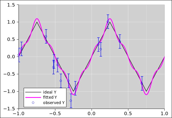 Figure 23
: Fitting a Fourier Series to Triangle-Wave Data
As implemented in reference 5, in cells
I24 through K38 we tablulate the basis functions. However,
this is just for show, and these tabulated values are not
used by the linest(...) function. You could
delete these cells and it would have no effect on the calculation.
Instead, the linest(...) function evaluates the
basis functions on-the-fly, using the array constant trick
as discussed in reference 7.
As always, the linest(...) function returns the fitted
coefficients in reverse order. In contrast, we really prefer to have
the coefficients in the correct order, as given in cells I9 through
K9, so that they line up with the corresponding basis functions in
cells I24 through K38. Alas there is not, so far as I know, any
convenient spreadsheet function that returns the reverse of a list,
but the reverse can be computed using the index(...) function,
as you can see in cell I9.
The linest(...) function can also return information about the
residuals and the overall quality of the fit. To enable this feature,
you need to set the fourth argument of linest(...) to
true. You also need to arrange for the results of the
linest(...) to fill a block M columns wide and 5 rows high,
where M is the number of basis functions; for example, M=2 for a
two-parameter straight-line fit. That is, highlight a block of the
right size, type in the formula, and then hit <ctrl-shift-enter>.
6 Uncertainty
We need to estimate the uncertainty associated with the fitted
parameters. The procedures for doing this in the linear case are
almost identical to the nonlinear case. See reference 8.
7 References
-
-
John Denker,
“spreadsheet for density determination”
./systematic-error-peculiar.xls
-
John Denker, “Twenty Questions”
www.av8n.com/physics/twenty-questions.htm -
John Denker,
“spreadsheet for measuring spring constant by observing period”
./measure-k-oscillator.xls
-
John Denker,
“Introduction to Probability”
www.av8n.com/physics/probability-intro.htm -
John Denker,
“spreadsheet demonstrating multi-parameter least-squares fitting
using nonlinear basis functions”
./linear-regression.xls
-
The Gnumeric Manual : LINEST
http://projects.gnome.org/gnumeric/doc/gnumeric-function-LINEST.shtml -
John Denker,
“Spreadsheet Tips and Techniques”
www.av8n.com/physics/spreadsheet-tips.htm -
John Denker,
“Nonlinear Least Squares”
www.av8n.com/physics/nonlinear-least-squares.htm