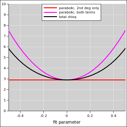
Figure 1: Chi-Square versus Fit Parameter
Least-square fitting it is used for fitting a theoretical curve (model curve) to a set of data. This is by no means the most general or most sophisticated type of data analysis, but it is widely used because it is easy to understand and easy to carry out.
The special case of linear least squares is discussed in reference 1.
We choose an objective function to be minimized. In general, we denote the objective function by є. For now, we choose it to be equal to the chi-squared.
| (1) |
where w specifies the weights, p is the vector of parameters, xi is the observed abscissa for the ith point, yi is the corresponding observed ordinate, and F is the fitted function. We care about χ2 because it is related to the negative log probability:
| (2) |
The constant of proportionality in equation 2 is the normalization constant, if you want your probabilities to sum to 1, which is usually not important. It corresponds to shifting the objective function by an irrelevant uniform additive constant. In contrast, the factor of −½ inside the exponential is important (and annoyingly easy to forget).
We will be interested in the first derivative:
| (3) |
where we have assumed that the w matrix is symmetric.
We will also need the second derivative:
|
The LHS is the second derivative (aka the Hessian) of the objective function. The term in square brackets in equation 4b is the second derivative (aka the Hessian) of the fitting function itself. These are not the same thing! In particular, if somebody starts talking about “the” Hessian you don’t necessarily know what they’re talking about.
Assuming the objective function is equal to the chi-square, once we have found it we can use it to calculate the covariance matrix for the fitted parameters. It’s just the matrix inverse:
| (5) |
At this point, if there are two or more fitted parameters, it pays to do a singular-value decomposition (SVD) of the covariance matrix. That’s because it is hard to understand the meaning of a matrix just by looking at it. SVD is a convenience in the 2×2 case, and a necessity for 3×3 or larger. In the present context, singular value decomposition is the same thing as eigenvalue decomposition (EVD). Looking at the eigenvalues and eigenvectors of the covariance matrix is a lot more informative than looking at the covariance matrix in its undecomposed form.
Recently I was doing a least-squares fitting exercise. The fit was behaving badly, so I suspected there was something fishy going on. However, before doing the SVD, I couldn’t have given a cogent explanation of the problem. After doing the SVD, it was easy to say that the covariance matrix was very nearly singular. The large eigenvalue was five and a half orders of magnitude larger than the small eigenvalue.
For more about SVD and its application to covariance matrices, see reference 2.
It is important to calculate the uncertainty associated with the fitted parameters. In the multi-parameter case, if the parameters are normally distributed, there will be a covariance matrix, as given by equation 5. In the single-parameter case, this reduces to a simple “error bar” associated with the parameter.
The RHS of equation 4 contains two terms: The term on the RHS of equation 4a is second degree, involving the product of two first derivatives. Meanwhile, the term in equation 4b is second order, involving the first power of a second derivative.
For linear least squares, the second-order term (equation 4b) vanishes ... but for nonlinear fitting it definitely does not. We shall see an example of this in a moment.
Remark: The second-degree term (equation 4a) is bilinear. It can be interpreted as the inner product between two Jacobians, using the weighting function w as a peculiar metric. However, I’m not sure this interpretation has much value, especially for non-linear fitting, where we have to worry about the second-order term in equation 4b, which cannot be put into bilinear form.
Example: Suppose we have a device that estimates velocity based on the rate at which heat is produced in a small brake. There is only one fitting parameter, namely the velocity itself. We observe the rate of heat production, which our model says should be proportional to velocity squared. Now imagine that under some circumstances, the brake is observed to be losing a tiny amount of heat. This tells us that our model is imperfect. That’s OK; in the real world, models are never perfect. Our model is not off by much, so let’s keep it. Let’s fit it to the data as well as can be. We anticipate that the best-fit value for the velocity will be zero. However, let’s turn the crank on the analytic machinery, to check that it gets the right answer. In any case, we need the machinery in order to calculate the associated uncertainty, which is not particularly obvious in advance.
The spreadsheet for producing these figures can be found via reference 3.
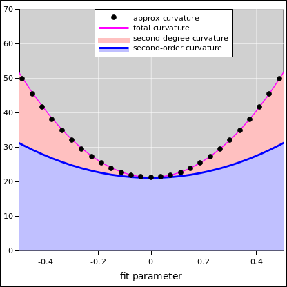
We need the second derivative of the objective function in order to estimate the uncertainty. In the neighborhood of the right answer (namely zero velocity), the second-order term in equation 4b tells the whole story. The bilinear term in equation 4a is provably zero at this point in parameter space. As you can see in figure 2, at the best-fit point 100% of the curvature comes from the second-order term. Even when we get moderately far from the best-fit point, the second-order contribution (as indicated by the light blue shaded region) is still the lion’s share of the total curvature (light blue plus pink).
| Insofar as the curvature isn’t constant, we shouldn’t be doing least squares at all. The parameter-values aren’t normally distributed. | However, in the neighborhood of the best-fit point, the curvature of the objective function is approximately constant, and we ought to use the correct constant! |
| You can see in figure 1 that a parabolic model (shown in magenta) does not exactly track the actual χ2 (shown in black), no matter what curvature we use. | If we include both terms in equation 4, the parabolic model (shown in magenta) is a reasonably decent approximation. |
In any case, the main point is that including both terms gives us a much better approximation than the second-degree term alone. That term predicts zero curvature, as shown in red in figure 1, which is just ridiculous. It corresponds to infinite error bars on the fitted parameter.
This simple example is not the only way of doing things. At some point, we should consider using a different model. For example, we could fit to the heat directly, and then take the square root of the fitted parameter. This would simplify the fitting process, which might or might not be the right thing to do. Remember, our primary objective is to get the right answer. One factor in the choice of models depends on whether we think the heat readings are normally distributed, or whether the velocities themselves are normally distributed.
This example was constructed to demonstrate that it is not hard to find situations where the second-order term in equation 4 cannot be neglected.
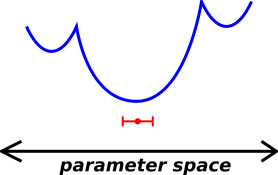
This term is all-too-often neglected, even when it shouldn’t be. Here is one way to understand how this mistake can arise. In linear least-squares fitting, the assumption of linearity is used twice: Once to find the best-fit parameters, and again when evaluating the uncertainty surrounding those parameters. In nonlinear least-squares fitting, everybody accounts for the nonlinearity when finding the best-fit parameters ... but then the all-too-common practice is to revert to linear thinking when estimating the uncertainty. Sometimes you can get away with this (as in figure 3), but sometimes you can’t.
I reckon there are three main cases to consider:
|
| |
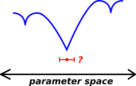
| Figure 3: Nonlinear Landscape, but More-Or-Less Linear Locally | Figure 4: Seriously Nonlinear Landscape | |
Therefore I recommend the following three-step procedure
Note that even if the observed y values are normally distribted, and even if they are independent i.e. uncorrelated, the best-fit parameter values could be strongly correlated.
Whenever we are at a minimum (possibly a local minimum) of the objective function є (considered as a function of p), the following zero-slope condition holds:
| (6) |
This is a necessary but not sufficient condition. A maximum of the objective function is not the best fit, indeed it is locally the worst fit, but it does satisfy equation 6.