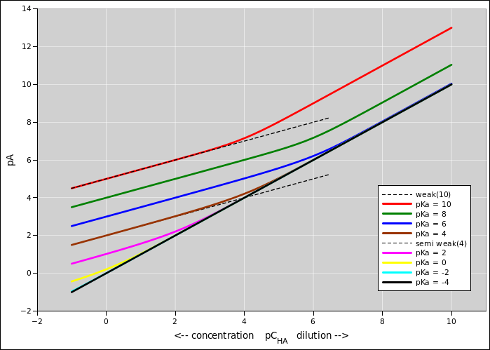
Figure 1: pH versus Concentration for Various pKa Values
Figure 1 shows pH as a function of concentration, for various pKa values, including weak acids and strong acids, as well as intermediate-strength acids, which are particularly interesting.
The pKa values for some common acids and bases are tabulated in reference 1 and reference 2. In this document, we consider only monoprotic acids.
These curves have a number of interesting properties:
| (1) |
where Ta is the total amount of acid in all its forms (ionized fully, partially, or not at all). For an explanation of other notation used here, see reference 3 or reference 4.
If we express the same relationship in terms of concentration (rather than log concentration) we get:
| (2) |
| (3) |
To say the same thing in other words: It is interesting that over the whole range from pKa = 0 to pKa = 5 or 6, the acid follows the weak-acid rule at high concentration, but then follows the strong-acid rule at moderately low concentration.
The meaning of equation 3 is clear: it just says that all the acid molecules are ionized (and that auto-ionization of the water molecules is negligible). This is what we expect for a reasonably concentrated strong acid ... and it also makes sense for a moderately-dilute moderately-weak acid. Simple entropy considerations suggest that greater dilution favors greater ionization.
| (4) |
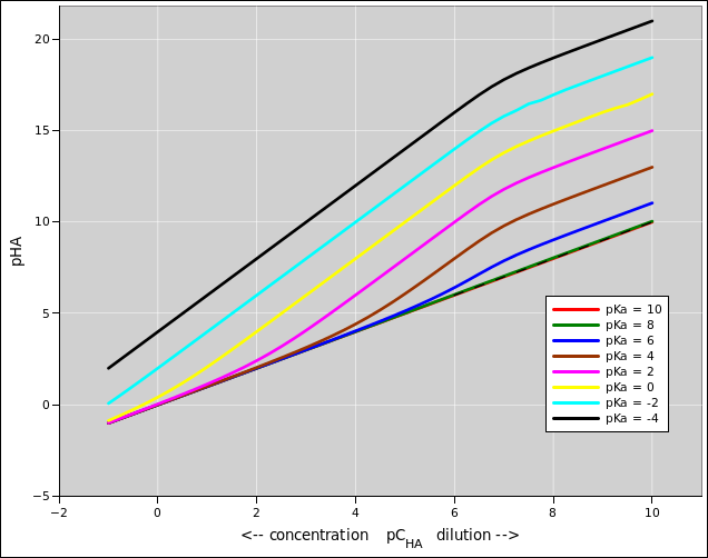
It is also interesting to see how much of the acid is ionized. This is shown in figure 2.
If we know [H+], we can find [A−] relatively easily. (Hint: combine equation 12 and equation 14.)
| (5) |
so the ionization percentage is:
Equation 6b is a tight bound for a dilute solution of a very weak acid (pKa = 7 or higher). The pH of the solution will never be less than the pH of water, so it’s clear the acid will never be 100% ionized, even when it very dilute. For example, if the pKa is 9, it will approach 1% ionization when it is very dilute.
Remark: This can be nicely explained as a common-ion effect.It is easy to find references that assert that any acid, no matter how weak, will be 100% ionized if it’s dilute enough. And it’s easy to see why people would make that mistake. In a vacuum, anything will dissociate if it’s dilute enough. As a famous example, hydrogen atoms in thermal equilibrium at 4 kelvin in outer space are ionized, simply because there is so much phase space for the particles to wander around in. Saha equation.
In contrast, our beaker of acid is not a vacuum. The presence of water guarantees that the H+ concentration never drops below 10−7 no matter how dilute the acid is. Those H+ ions push the equilibrium to favor the unionized HA molecule.
The common-ion effect is commonly expressed as a “solubility” issue, but really it’s an ionization issue. The distinction is important if the unionized species is reasonably soluble. A good example is boric acid, pKa = 9.5.
Equation 6b is also a tight bound for a sufficiently concentrated solution of a weak acid, even if it’s not very weak. In such cases we have:
| (7) |
The amount of unionized acid is:
| (8) |
so the percentage is:
| (9) |
We can do the same for the amount of unionized acid:
The curves in figure 1 were computed by solving the following equation. It is a cubic polynomial, with one positive root and two negative roots. The positive root is the only one that makes sense as a concentration.
| (10) |
This works for strong acids, weak acids, and everything in between, provided it is a monoprotic acid. It can be considered a simplified version of equation 46, applicable when there are no other acids or bases in the system.
As a check on the algebra, you can set Ka=0 in equation 10, in which case [H+] = √Kw as it should.
It is easy to solve equation 10 with an iterative root-finding algorithm. I’ve had good luck with the Brent algorithm (reference 5).
In contrast, beware that standard “algebraic” formulas for solving the cubic can give wrong answers in some cases. Depending on details of the implementation, the formulas can be numerically unstable. That is to say, the result gets trashed by roundoff errors. Specifically: I tried using the standard library routine gsl_poly_complex_solve_cubic() and it failed spectacularly for certain values of pKa and pTa. Some of the alleged results were off by multiple orders of magnitude. Some of the alleged results were complex numbers, even though the right answers were real numbers. It might be possible to rewrite the code to make it behave better, but that’s not a job I’m eager to do.
Lesson #1: Something that looks like an “exact” closed-form solution might not be at all suitable for real-world numerical calculation ... whereas an approximate, iterative solution might be highly accurate in practice.
Lesson #2: The failure of the algebraic method serves as a reminder of the difference between uncertainty and significance. The inputs to the method might or might not be uncertain; it doesn’t actually matter. The output (i.e. the root as plotted in figure 1) has a tolerance of a few percent. The internal calculations use IEEE double-precision floating point, which is good to about 16 decimal digits ... which is not enough for the task at hand. Even though the tolerance allows uncertainty in the second digit, there is significance in the 16th digit and beyond. So, if you see a number of the form:
| (11) |
you should not assume it is safe to round things off. In this case, such a number already has too few digits. For more on this, see reference 6.
The C++ code to calculate the pH as a function of concentration can be found in reference 7.
Here is a quick summary of the starting point and the ending point. We postpone to section 4.3 the details of the intermediate steps. For an explanation of the notation used here, see reference 3 or reference 4.
For starters, we need the definition of the acid dissociation constant:
| (12) |
and similarly the water dissociation constant:
| (13) |
We also need the conservation laws, including conservation of A-groups in our acid:
| (14) |
as well as conservation of charge:
| (15) |
That gives us four equations in four unknowns. Turning the crank on the algebra gives us:
| (16) |
which is the same as equation 10.
|
And the two conservation laws:
|
That gives us five equations in five unknowns. We can flip each line of equation 17:
| (19) |
and use that to eliminate 3 of the 5 unknowns from equation 18:
| (20) |
Isolate factors of 1/[H2A] :
|
Use equation 21a to eliminate [H2A] from equation 21b:
| (22) |
Multiply by [H+]3 Ta to get rid of all denominators:
| (23) |
We can check that when Ka2 is zero, that reduces to:
| (24) |
which is the same as equation 10.
To obtain [H2A] we rewrite equation 21a as:
| (25) |
To obtain [HA−] we rewrite equation 17a as:
| (26) |
To obtain [A] we rewrite equation 17b as:
| (27) |
Similarly:
| (28) |
And then we can plug into equation 18 to close the loop and verify that our calculations are correct. This serves to:
Let’s create something that might serve as a buffer solution. We start with the acid considered in section 4.1, and also add a certain amount of very strong base (EOH!). The buffer doesn’t require it, but let’s also add a certain amount of very strong acid (H@!).
We call HA the main acid, to distinguish it H@!. For a practical buffer, it should be a weak acid, but the equations in this section are the same whether it is weak or not.
As in equation 12 the acid dissociation constant is:
| (29) |
As in equation 13 the water dissociation constant is:
| (30) |
As a slight generalization of equation 14, the A-groups coming from our main acid are conserved:
| (31) |
At this point, we add a new equation, stating that the E-groups coming from the strong base are conserved:
| (32) |
Similarly the @-groups coming from the strong acid are conserved:
| (33) |
Since we are assuming the strong base and strong acid are very strong, we can immediately simplify the three previous equations to:
| (34) |
and
| (35) |
and
| (36) |
Charge is conserved. This is like equation 15, except that now we have to include the strong base and the optional strong acid:
| (37) |
or, simpler:
| (38) |
where σ is the net charge floating around from the strong base and/or acid:
| (39) |
Now we turn the crank. We start by plugging into equation 29, using equation 34 to eliminate the unknown [HA] from the system of equations.
That gives us
| (40) |
hence:
| (41) |
hence:
| (42) |
We now plug into the charge-conservation expression, equation 38, using equation 35, equation 42, and equation 30 to get rid of all the unknowns. That gives us
| (43) |
Multiplying through by [H+] gives us
| (44) |
Multiplying through by the remaining denominator gives us:
| (45) |
Note that this introduces a spurious root at [H+] = − Ka whenever Ka and/or Ta is zero. Knowing this will be useful in a moment.
The equation can be rearranged to give the “usual” result:
| (46) |
The product of the roots is positive, and we know one root is negative, so the other two must have opposite signs. Therefore overall there is one positive root and two negative roots.
By setting (Ceoh! − Ch@!) to zero we obtain equation 10, so you can see why we didn’t bother deriving it directly; it is easier to do the more-general case and specialize to (Ceoh!−Ch@!)=0 later.
As a check on the algebra, you can set Ka=0, in which case equation 46 simplifies to:
| (47) |
Let’s check what this says about a strongly acidic solution. That means (Ceoh! − Ch@!) is large and negative. Therefore [H+] is large. The first two terms in equation 47 dominate, and [H+] converges to Ch@!, as it should.
Let’s also check what this says about a strongly basic solution. That means (Ceoh! − Ch@!) is large and positive. Therefore [H+] is small. The last two terms in equation 47 dominate, and [H+] converges to Kw/Ceoh!, as it should.
As an even more incisive check on the equations, we should consider the case where half of the main acid is ionized. This is discussed near the end of section 4.4.
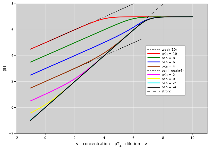
It is sometimes convenient to restrict attention to the parts of figure 1 that are not too near the top. That is, we focus attention on solutions that are definitely acidic, with a pH well below the pH of water. In this case, equation 10 simplifies to:
| (48) |
as you can see by starting with equation 10 and setting Kw to zero. Equation 48 can also be easily derived directly from equation 12, equation 14, and the simplified charge-conservation law:
| (49) |
Equation 48 is a quadratic polynomial. It has one positive root and one negative root. We care about the positive root, namely
| (50) |
For a strong acid (large Ka), equation 50 simplifies to
| (51) |
as expected.
For a suffciently high concentration of a weak acid, equation 50 simplifies to
| (52) |
In other words, the pH is the geometric mean between the concentration and the acid dissociation constant. For example, acetic acid has a pKa of 4.75. Now 1.78 millimolar acetic acid has a pC of 2.75, so it should have a pH of 3.77 according to equation 50, or approximately 3.75 as estimated by equation 52, so the latter is off by less than one percent.
Within the regime where equation 52 is valid, as you increase the concentration, the pH drops, but only slowly. For each factor of 10 in the concentration, the pH drops by only half a unit, not a full unit, because of the square root in equation 52.
Beware that the range of validity does not extend to the point where the two factors on the RHS of equation 52 are equal. That is, at the point where the concentration is equal to the Ka, equation 52 might suggest that the pH would be equal to the pKa, but the reality is otherwise. You need at the concentration to be at least two orders of magnitude larger than Ka before the equation is reliably valid.
As another amusing corollary, when pH equals pKa, exactly half of the substance is ionized. That is, the ionized [A−] is equal to the unionized [HA] in accordance with the fundamental definition, equation 12.
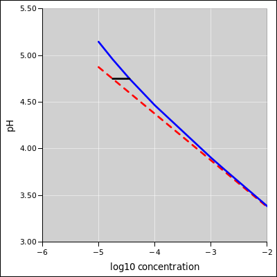
If you want to achieve pH equal to pKa, the concentration needs to be very nearly twice the Ka, as you can see from equation 48. This is nice to know. Also it tells you that equation 52 is off by a factor of 2 in this regime. See figure 4.
As yet another corollary, when designing a pH buffer system, it makes sense to operate near pH = pKa. Typically this means adding rather a lot of weak acid (concentration more than Ka) and then raising the pH back to pKa by adding some strong base.
In the figure, the blue line is the more-accurate prediction, equation 50, while the red dashed line is the less-accurate prediction, equation 52. The height of the black tie-line corresponds to pH = pKa. The length of the line is 0.301 common-logarithmic units, which corresponds to a factor of two in concentration.
It must be emphasized that all the results in this section, including figure 4, assume that the acid is not unduly weak. It needs to be strong enough so that the H+ ions it contributes are the dominant contribution (dominating over the water contribution), even when it is only half ioinized. For more about the range of validity, see section 4.5.
Let’s investigate the range of validity of the approximations used in section 4.4. In this section we don’t assume low pH; we use the more general equations to see what happens at low and not-so-low pH.
We define x to represent the situation where [H+] = Ka = x and Ta = 2x. We plug this into the RHS of equation 53, and see how close it comes to being a root. We rewrite equation 10 as:
| (53) |
Taking the derivative we find:
| (54) |
Plugging in the definition of x we get:
| (55) |
From this we conclude that at pH 6 or below, the approximation leading to equation 48 should get the concentration right within a percent or so. At higher pH you have to use the full cubic.
Let’s consider a system that is the same as in section 4.3, except that we consider a weak base (rather than a weak acid) plus a strong base (EOH!). The buffer doesn’t require it, but we also include a certain amount of strong acid (H@!).
The weak base dissociation constant is:
| (56) |
As always, the water dissociation constant is:
| (57) |
The B-groups are conserved in our weak base:
| (58) |
Similarly, the @-groups are conserved:
| (59) |
And the E-groups are conserved:
| (60) |
Since we are assuming the acid and strong base are very strong, we can immediately simplify this to
| (61) |
and
| (62) |
and
| (63) |
As always, charge is conserved:
| (64) |
Now we turn the crank. We start by plugging into equation 56, using equation 61 to eliminate the unknown [BOH] from the system of equations.
That gives us
| (65) |
hence:
| (66) |
hence:
| (67) |
We now plug into the charge-conservation expression, equation 64, using equation 67, equation 62, and equation 57 to get rid of all the unknowns. That gives us
| (68) |
Multiplying through by [H+] gives us
| (69) |
Multiplying through by the remaining denominator gives us
| (70) |
If you want a monic polynomial, it is probably better to use equation 74, but if Kb is nonzero you could consider rewriting equation 70 as a monic polynomial:
| (71) |
Notice that the results are not sensitive to the concentration of strong base and strong acid separately, but only to the net difference between the two.
By setting (Ceoh! − Ch@!) to zero we obtain the simpler expression:
| (72) |
As a check on the algebra, you can set Kb to zero in equation 72, in which case [H+] = √Kw as it should.
As an even more incisive check on the algebra, solve for [OH] instead. The first step is:
| (73) |
which simplifies to:
| (74) |
which is the mirror image of equation 46.