Figure 1: Phase Space of a Harmonic Oscillator
In typical applications, such as for finding a numerical solution to the equations of motion, a symplectic integrator often works very much better than a non-symplectic integrator.
Our task for today is to vizualize what’s going on, and to understand why the properties that make the integrator symplectic also make it good.
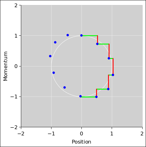
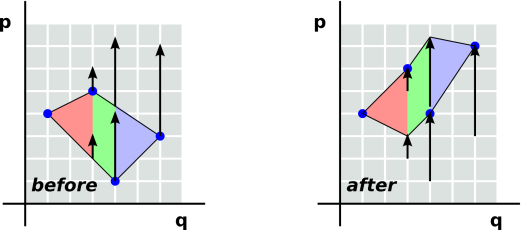
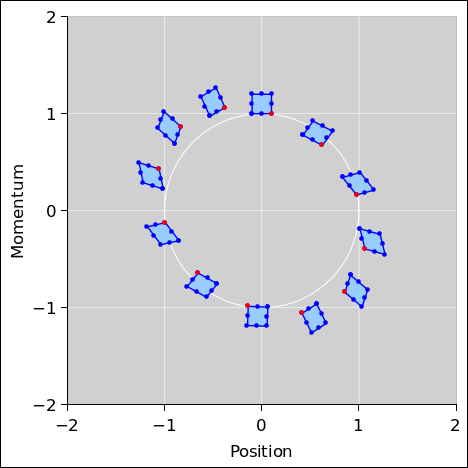
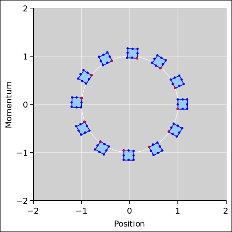
Figure 1 is a phase-space plot showing the dynamics of a simple harmonic oscillator. This is a reasonably accurate representation of the real physics.
We start with an ensemble of eight oscillators and then show the time-evolution of the ensemble. The initial conditions are such that all eight systems start out near the 12:00 position in the figure. After the first time-step, they are all near the 1:00 position, and so forth, clockwise.
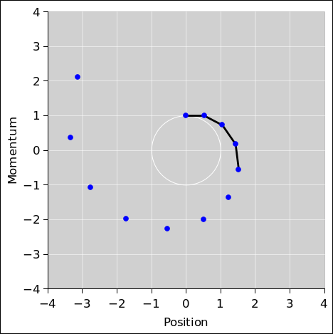
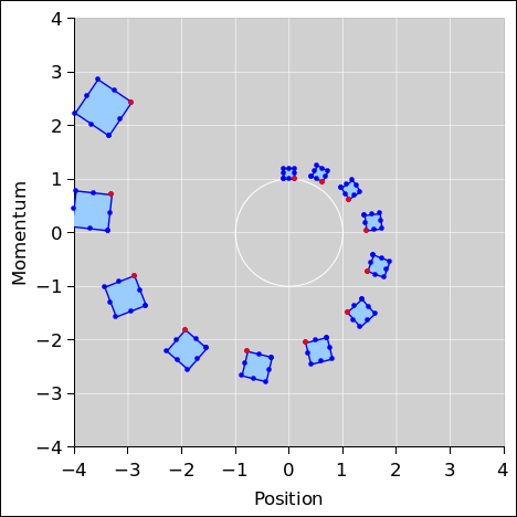
Figure 2 is a phase-space plot showing the results of a first-order symplectic integrator applied to the equations of motion for a harmonic oscillator. Ideally this would be the same as figure 1; however we have chosen to use a low-order integrator with a large step size, so that we can visualize some of the advantages and limitations of the method. The spreadsheet used to produce these figures is cited in reference 1. Some C++ code to perform symplectic integration is cited in reference 2.
|
| |
| Figure 2: Symplectic Integration : Harmonic Oscillator | Figure 3: Non-Symplectic Integration : Harmonic Oscillator | |
You may have heard that a symplectic integrator “preserves area in phase space” or something like that. More specifically:
In figure 2, the symplectic integrator conserves the area of the little blue boxes. The boxes change shape, but their area stays the same.
As a not-very-useful corollary, for a periodic system, there is another area that is conserved, namely the area inside the phase-space orbit of the system. Proof: Choose an ensemble of systems that are time-delayed versions of each other, such as the ensemble consisting of all the red dots in figure 2 (along with more red dots of the same kind, to fill in the gaps). This ensemble marks out an orbit for you. Alas this is not very interesting or useful, so far as I know, because the orbit has no dynamics. It just sits there. So, the fact that its area is conserved doesn’t tell us anything we didn’t already know.
The trivial dynamics covered by this corollary stands in contrast to the highly nontrivial dynamics of the little blue-filled squares in figure 2. The main reason for mentioning the orbit is to make the point that there are lots of different things with dimensions of area in phase space. Some are conserved and some not. Some are interesting and some not. You have to specify which sort of area you are talking about.
Let’s consider, one by one, a few of the key properties of the real harmonic oscillator as shown in figure 1, in comparison to the two integration schemes we are considering, as shown in figure 2 and figure 3.
On the other hand, at the end of each cycle, the symplectic solution returns to the same energy. We assert without proof that over the long term, the energy error remains bounded (in a periodic system).
Here we are considering only the error contributed by the coarseness of the time-step. (There will be additional errors contributed by roundoff, i.e. associated with machine precision, but they are very small unless you are taking huge number of steps. We will have nothing more to say about machine precision in this document.)
In this section we restrict attention to various versions of the first-order Euler integrator. For most practical applications, you would be better off with a higher-order integrator. See section 6 for more about this.
Let’s compare the symplectic version to the non-symplectic version of first-order Euler. We can use various methods – diagrams, equations, and code – to help understand what’s going on.
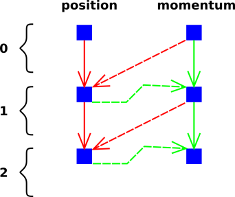
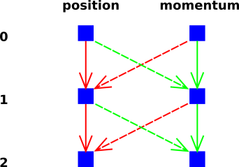
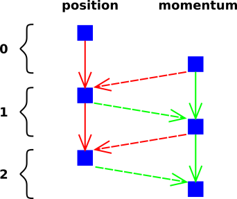
| The symplectic update rule has an alternating pattern as shown in figure 4. | The forward Euler rule has a criss-cross, non-staggered pattern, as shown in figure 5. |
In both of these figures, each diagonal dashed arrow represents an update, proportional to the timestep Δt. Meanwhile, each vertical solid arrow represents the simple memory of the previous coordinate (position or momentum). The memory plus the update determine the new coordinate.
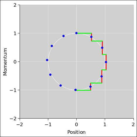
| Figure 6 shows what this looks like in phase space. Starting at 12:00, we first update the position (as shown by a horizontal green line). Then we update the momentum (as shown by a vertical red line). The change in momentum is calculated based on the latest updated position. | In figure 7, the position and momentum are updated at the same time. The change in momentum is calculated based on the position as it was before this update. |
We can understand even more if we treat [p, q] as a vector in phase space. The crucial property of the symplectic integrator’s first half-step equation 3 concerns the magnitude and the direction of the update. The direction is entirely in the q direction, while the magnitude is independent of q. The magnitude is a function of p only.
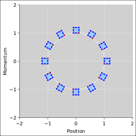
Similarly, in equation 5, the direction of the update is entirely in the p direction, while the magnitude is a function of q only. This is diagrammed in figure 8. The situation before the update is shown on the left, while the situation after the update is shown on the right. We divide the initial quadrilateral into a collection of triangles and trapezoids, all with their bases aligned vertially, i.e. aligned along contours of constant q. The update rule slides each base parallel to itself, without changing the length, because the Δp is a function of q only.
Recall the formula for the area of a trapezoid, namely one half of the sum of the bases times the altitude. A triangle is just the limiting case of a trapezoid with one really small base. As a corollary, if you slide a base parallel to itself, it does not change the area.
Note that in figure 8, all the bases run vertically and all the altitudes run horizontally. The terminology is a bit ugly, but it is conventional, so we are sticking with it.
So, we begin to see the origin of the crucial property of the symplectic integrator. The update rules are guaranteed to conserve area in phase space.
A sufficient way to achieve this is to have the p-update be a function of q only, and the q-update be a function of p only. (There are other ways of conserving area, but this one is particularly easy to understand and to visualize.)
Note the contrast:
| Area: | The symplectic integrator conserves area in phase space exactly. | |
| Area is conserved no matter how large or how small the step-size. | ||
| Energy: | The symplectic integrator conserves energy only approximately. | |
| The energy error gets smaller as the step-size gets smaller. |
If you just look at the code, the difference between symplectic and non-symplectic is so small that if you blink you’ll miss it.
| The update rule for the “symplectic Euler” algorithm looks perfectly reasonable: | The update rule for the corresponding old-fashioned (non symplectic) “forward Euler” algorithm also looks perfectly reasonable, even though it does not work nearly so well: |
|
|
| The symplectic algorithm updates the momentum by integrating over the backward interval, using the force law at the new position. | The forward Euler algorithm updates the momentum by integrating over the forward interval, using the force law at the old position. |
| Meanwhile, both algorithms update the position by integrating over the forward interval, using the velocity at the old position. |
To summarize, the symplectic algorithm is in some sense half forward, half backward. However, that’s not really the best way to think about it. We are better off if we rewrite each of the previous equations, not changing the meaning, but improving the clarity by breaking each symplectic step into two half-steps, and trying to do the same for each non-symplectic step.
The first half-step updates the position q.
|
|
The second half-step updates the momentum p:
|
|
| The crucial property of the sympletic integrator is that the position is updated by an amount that depends only on the current momentum, and then the momentum is updated by an amount that depends only on the current position. | In the non-symplectic integrator, both updates occur at the same time. There isn’t a clean way to break the update into two steps, because p(1b) depends on the original q(0), not the current q(1a). |
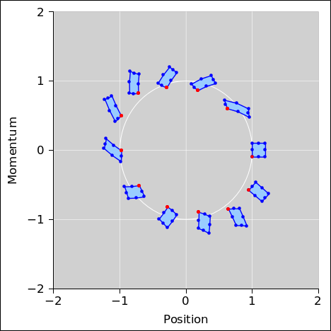
Figure 9 is pretty much the same as Figure 2, except that the oscillator’s force law is slightly anharmonic. Because of the anharmonicity, the shape of the ensemble necessarily changes as a function of time. However, the area remains constant. The symplectic integrator handles this case just fine.
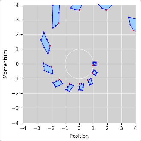
Figure 10 shows the non-symplectic forward Euler algorithm applied to the same oscillator.
|
| |
| Figure 9: Symplectic Integration : Anharmonic Oscillator | Figure 10: Non-Symplectic Integration : Anharmonic Oscillator | |
Note that the forward Euler algorithm we are using here can be considered “standard” but not very sophisticated. It is possible to improve it ... but it is hard to improve it very much with out “accidentally” making it symplectic.
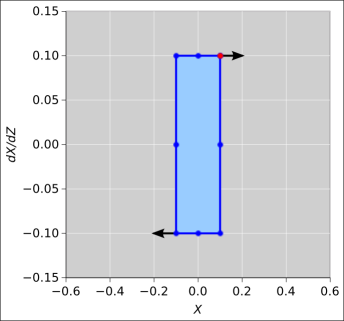
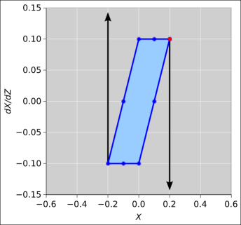
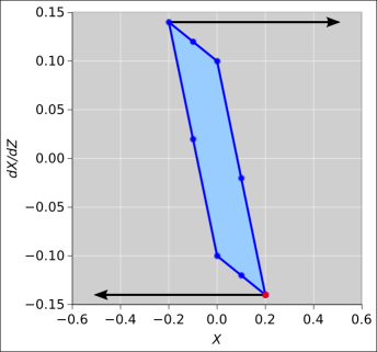
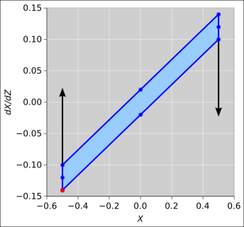
Consider an optical system consisting of thin lenses, with the optical axis running in the Z direction. The axes in phase space are X and dX/dZ. The equations of motion are simple:
In each of the following figures, the blue shaded area represents the phase space at a certain stage, and the black arrows represent change the necessary to reach the next stage.
We see that the update of X is independent of X, and the update of dX/dZ is independent of dX/dZ. This is sufficient to guarantee that area in phase space is conserved.
For the next level of detail on this, see reference 4.
Let’s discuss block ciphers. Modern ciphers consist of multiple stages, called rounds. Each round transforms the block of data in some way.
Suppose that at each state, the transformation involves splitting the block into two pieces X and Y, and then updating X based on some function that depends on Y but is independent of X. In the simplest case, Y is then updated using some function that is independent of Y.
| (7) |
A round that behaves like this is said to have the Feistel property.
This property is sufficient to guarantee that the round is reversible. If all rounds have this property, it guarantees that the cipher can be deciphered by anyone who knows the key, no matter what the f and g might be doing. Indeed enciphering and deciphering are almost identical, requiring little more than reversal of the key schedule.
To say the same thing in other words, a Feistel round is guaranteed to leave the entropy (and information) unchanged.
Without the Feistel property, it might be hard to prove that the round function was invertible even in principle, and even harder to compute the inverse.
The Velocity Verlet method is second-order and symplectic. This stands in contrast to the method considered in section 3, which is symplectic but only first order. The advantage here is higher accuracy. If your errors were on the order of 10−5 with a first-order method, they will be on the order of 10−10 with a second-order method.
There exist even higher-order symplectic integrators, fourth-order and beyond. These allow you to take a larger step size while maintaining high accuracy. The drawback is that the equations are more difficult to understand and more complicated to implement. At some point you should switch to using a professionally-designed “canned” higher-order integrator, but first it is worth experimenting with first-order and second-order methods long enough to gain an understanding of what’s going on.
Here’s an example of a second-order symplectic integrator, namely the Velocity Verlet method applied to the simple harmonic oscillator. The basic idea is the same as plain old first-order Euler, except that the velocities are evaluated at times that are shifted half a step relative to the positions. You can see this by comparing figure 15 to figure 4.
| This second-order method goes by many names. Among other things, it is often called the leapfrog method, which is meant to evoke the alternating structure of figure 15. | In contrast, when playing leapfrog, it would be a bad idea to have both frogs jumping at the same time, as in figure 16. |
In typical applications, the second-order integrator is orders of magnitude more accurate compared to the first-order integrator, as you can see by comparing figure 17 to figure 18.
|
| |
| Figure 17: Second-Order Symplectic Integration : Harmonic Oscillator | Figure 18: Symplectic Integration : Harmonic Oscillator | |
As before, we are assuming the force depends only on position. This rules out frictional forces and anything else that depends on velocity.
Here is the most prosaic way of writing the Velocity Verlet update equations:
| (8) |
The physics here makes sense: The position x crosses the interval from x(0) to x(1) using the velocity in the middle of the interval, namely v(½). The velocity v crosses the interval from v(0) to v(1) using the average acceleration, namely half of the initial acceleration plus half of the final acceleration.
Let’s look at two iterations:
| (9) |
The steps are shown in figure 19. We can understand what makes the system symplectic, as follows: Start from the point at the 1:00 position. We first update the momentum half a step, as shown by the vertical red half-line descending from this point. This updates velocity based on position alone, so it preserves area in phase space. Next we update the position, as shown by the horizontal green line. This updates position based on velocity alone, so it also preserves area. Finally we update the velocity again, as shown by the vertical red half-line descending toward the new 2:00 point. This updates velocity based on the (new) position alone, so yet again, area is conserved.
We can improve our understanding the strategy of the second-order integrator as follows:
| Consider the Z-shaped steps that take us from point to point in the second-order integrator as shown in figure 19. These steps keep the system point close to where it belongs, i.e. close to the white circle. With unimportant exceptions, each green bar and each full red bar straddles the circle in a symmetric way. | Consider the L-shaped steps in the first-order integrator as shown in figure 20. These steps don’t stay close to the circle. If the points were on the circle, these steps would look even worse: The steps would be entirely outside the circle in the quadrant from 12:00 to 3:00 and entirely inside the circle in the quadrant from 3:00 to 6:00. |
| Here’s why the exceptions are unimportant: In figure 19 there is in principle a red half-line descending from the 12:00 point, but it has zero length, so you can’t see it. The key idea is that the acceleration (dv/dt) is zero at this point. This explains the zero-length red bar. Not coincidentally, the same idea explains why the green bar that starts at 12:00 ends at the correct place, correct to second order. It might look like it’s first order, but it’s also good to second order, because the second-order term (½at2) is zero. |
| The same logic explains why the red half-bar that starts at 3:00 ends at the correct place, correct to second order. |
We can make the calculation more efficient if we introduce a new variable, namely the advanced velocity:
| (10) |
That gives us:
| (11) |
Note that in the inner loop of the integration, you don’t need to evaluate v at all. In the inner loop, it suffices to evaluate x and w. Notice that in equation 11 we did not evaluate v(1).
On the other hand, you are free to evaluate v at some or all of the steps if you are curious about it. On all steps except the very last, a good estimate is:
| (12) |
Assuming you are given initial values for x and v but not w, you need to prime the pump, using a half-sized time step to evaluate w(1). This is done outside the inner loop. This step is first-order, not second-order. If you’re not careful, the error in this step could dominate the errors in all other steps combined. You might want to do something special with this. You might consider using more terms in the Taylor series to make it second-order. You might also consider starting the integration from t=−1 and choosing fake initial data (at t=−1) that is consistent with the real initial conditions (at t=0).
Once the pump has been primed, the inner loop just rolls along, updating x and w with no half-sized steps.
Here’s another reason why it was worth writing equation 11: It allows us to see that the update preserves area in the (x, w) plane. The position x is updated by an amount that depends only on w, and the advanced velocity w is updated by an amount that depends only on x.
Figure 21 is similar to figure 17, except that a 3× smaller step-size is used. The step-size is 10∘. Only every third step is plotted. That is to say, there are two invisible boxes in between each pair of visible boxes in figure 21.
Decreasing the step size by a factor of 3 reduces the phase error by a factor of 9, which is what we would expect from a second-order method. Specifically, the phase error goes from 71 milliradians per cycle to 8 milliradians per cycle.
In a practical application, the step size would be several orders of magnitude smaller than this.